Probability Biostatistics Dr Muhammad Arif Ph D m

Probability & Biostatistics Dr. Muhammad Arif, Ph. D m. arif@faculty. muet. edu. pk 由Nordri. Design提供 www. nordridesign. com

Course Outline • Introduction to Biostatistics • Descriptive Biostatistics • Probability • Discrete Probability Distributions • Continuous Probability Distributions • Sampling Distributions • Estimation • Hypothesis Testing

Lecture Outline • Simple Random Sampling • Sampling Distributions • Distribution of the Sample Mean • Central Limit Theorem • Distribution of the difference between two Means • Distribution of the Sample Proportion • Distribution of the difference between two Proportions

Introduction • Parameters are numerical descriptive measures for populations. • Two parameters for a normal distribution: mean µ and standard deviation σ. • One parameter for a binomial distribution: the success probability of each trial p. • Often the values of parameters that specify the exact form of a distribution are unknown. • You must rely on the sample to learn about these parameters.

Simple Random Sampling • The sampling plan or experimental design determines the amount of information you can extract, and often allows you to measure the reliability of your inference. • Simple random sampling is a method of sampling that allows each possible sample of size n an equal probability of being selected.

Sampling Distributions • Any numerical descriptive measures calculated from the sample are called statistics. • Statistics vary from sample to sample and hence are random variables. • This variability is called sampling variability. • The probability distributions for statistics are called sampling distributions.

Sampling Distributions The distribution of all possible values that can be assumed by some statistic, computed from samples of the same size randomly drawn from the same population, is called the sampling distribution of that statistic. • Sampling distributions are important in the understanding of statistical inference. • Probability distributions permit us to answer questions about sampling and they provide the foundation for statistical inference procedures.

Construction of Sampling Distributions Sampling distributions may be constructed empirically when sampling from a discrete, finite population. Note that this construction is difficult with a large population and impossible with an infinite population. To construct a sampling distribution we proceed as follows: 1. From a population of size N, randomly draw all possible samples of size n. 2. Compute the statistic of interest for each sample. 3. Create a frequency distribution of the statistic.

Important Characteristics of Sampling Distributions We usually are interested in knowing three things about a given sampling distribution: 1. its mean, 2. its variance, and 3. its functional form (how it looks when graphed).

Types of Sampling Distributions There are Four types of sampling distributions. 1. Distribution of the Sample Mean 2. Distribution of the difference between two Means 3. Distribution of the Sample Proportion 4. Distribution of the difference between two Proportions

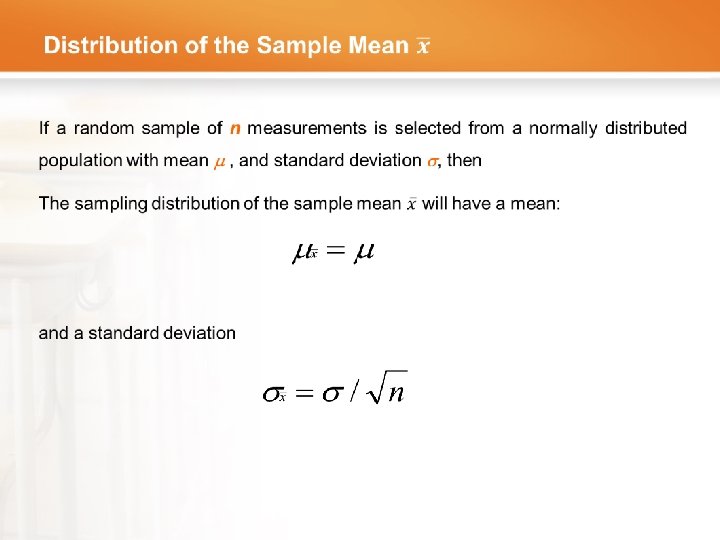
Standard Error The square root of the variance (or standard deviation) of the sampling distribution is also called the standard error of the mean or the standard error.

Sampling from Non-Normally Distributed Populations When the sampling is done from a non-normally distributed population, the central limit theorem is used.

Central Limit Theorem •

Central Limit Theorem • The Central Limit Theorem also implies that the sum of n measurements is approximately normal with mean nm and variance σ2/n . • Many statistics that are used for statistical inference are sums or averages of sample measurements. • When n is large, these statistics will have approximately normal distributions. • This will allow us to describe their behavior and evaluate the reliability of our inferences. • Note that the central limit theorem allows us to sample from non-normally distributed populations with a guarantee of approximately the same results as would be obtained if the populations were normally distributed provided that we take a large sample.

Central Limit Theorem •

Central Limit Theorem: When randomly sampling from any population with mean m and standard deviation s, when n is large enough, the sampling distribution of x bar is approximately normal: ~ N(m, s/√n). Population with strongly skewed distribution Sampling distribution of for n = 10 observations Sampling distribution of for n = 2 observations Sampling distribution of for n = 25 observations

Central Limit Theorem Example: Given the information below, what is the probability that x is greater than 53? Solution Data m = 50 s = 16 n = 64 P(x > 53) = ? Sketch a normal curve as shown in the figure. Convert x to a z score Continue on next slide…

Central Limit Theorem Find the appropriate value of Z in the table A value of z = 1. 5 gives an area of. 9332. This is subtracted from 1 to give the probability P (z > 1. 5) =. 0668 There the probability that x is greater than 53 is. 0668.

Central Limit Theorem Example: Suppose it is known that in a certain large human population cranial length is approximately normally distributed with a mean of 185. 6 mm and a standard deviation of 12. 7 mm. What is the probability that a random sample of size 10 from this population will have a mean greater than 190? Solution Data m = 185. 6 s = 12. 7 n = 10 P(x > 190) Sketch a normal curve as shown in the figure. Convert x to a z score Continue on next slide…

Central Limit Theorem • It is find that the area to the right of 1. 10 is. 1357; • hence, we say that the probability is. 1357 that a sample of size 10 will have a mean greater than 190.

Central Limit Theorem •

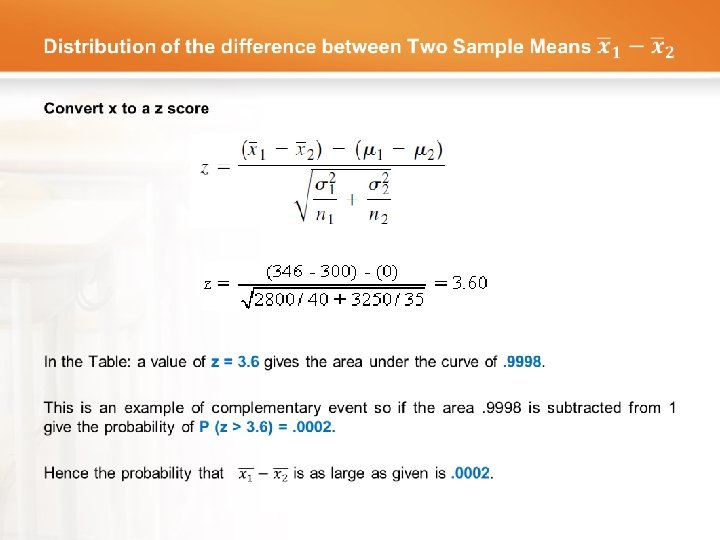
Converting x into z score The normal distribution can be transformed to the standard normal distribution using the formula as; We can find the z score by assuming that there is no difference between the population means.

• Continue on next slide…

While statistics such as the sample mean are derived from measured variables, the sample proportion is derived from counts or frequency data. Construction of the sampling distribution of the sample proportion is done in a manner similar to that of the mean and the difference between two means. When the sample size is large, the distribution of the sample proportion is approximately normally distributed because of the central limit theorem.

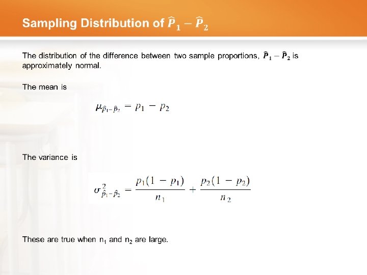
The Central Limit Theorem can be used to conclude that the binomial random variable x is approximately normal when n is large, with mean np and variance npq. The sample proportion, is simply a rescaling of the binomial random variable x, dividing it by n. From the Central Limit Theorem, the sampling distribution of a sample proportion will also be approximately normal, with a rescaled mean and variance p(1 - p)/n or pq/n. , A random sample of size n is selected from a binomial population with parameter p. If n is large, and p is not too close to 0 or 1, the sampling distribution of will be approximately normal.

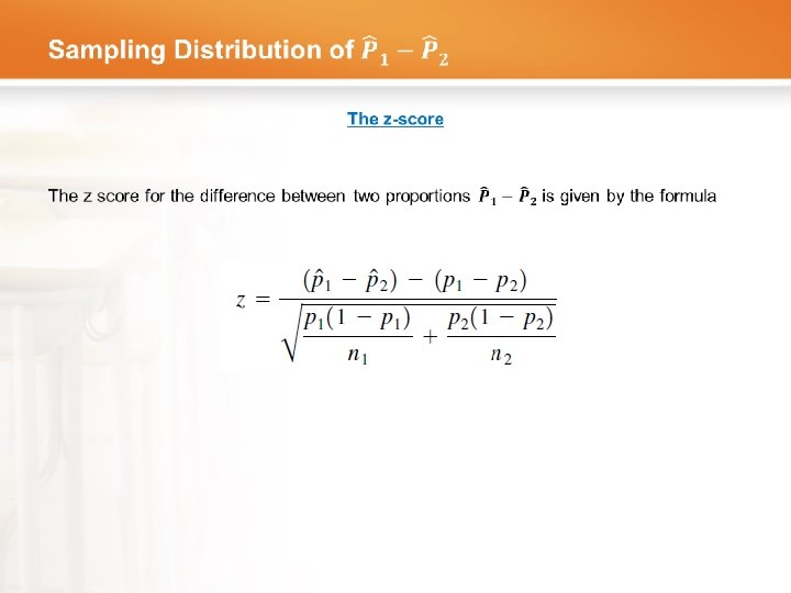
The z-score for the sample proportion is

Example: In the mid seventies, according to a report by the National Center for Health Statistics, 19. 4 percent of the adult U. S. male population was obese. What is the probability that in a simple random sample of size 150 from this population fewer than 15 percent will be obese? Solution Data n = 150 p =. 194 P( <. 15) = ? Sketch a normal curve as shown in the figure. Calculating the z score Continue on next slide…

When look at the table, we find that a value of z = -1. 36 gives an area of. 0869. Hence the probability that <. 15 is. 0869.

Example: Blanche Mikhail studied the use of prenatal care among low-income African-American women. She found that only 51 percent of these women had adequate prenatal care. Let us assume that for a population of similar low-income African-American women, 51 percent had adequate prenatal care. If 200 women from this population are drawn at random, what is the probability that less than 45 percent will have received adequate prenatal care? Solution

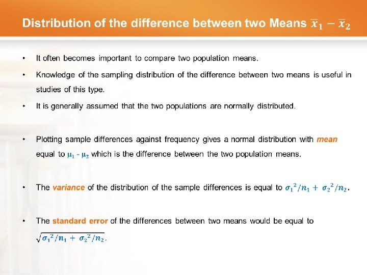
Distribution of the Difference Between Two Sample Proportions • Often there are two population proportions in which we are interested. • We desire to assess the probability associated with a difference in proportions computed from samples drawn from each of these populations. • The relevant sampling distribution is the distribution of the difference between the two sample proportions.

• The sampling distribution of the difference between two sample proportions is constructed in a manner similar to the difference between two means. • Independent random samples of size n 1 and n 2 are drawn from two populations of dichotomous variables where the proportions of observations with the character of interest in the two populations are p 1 and p 2, respectively.

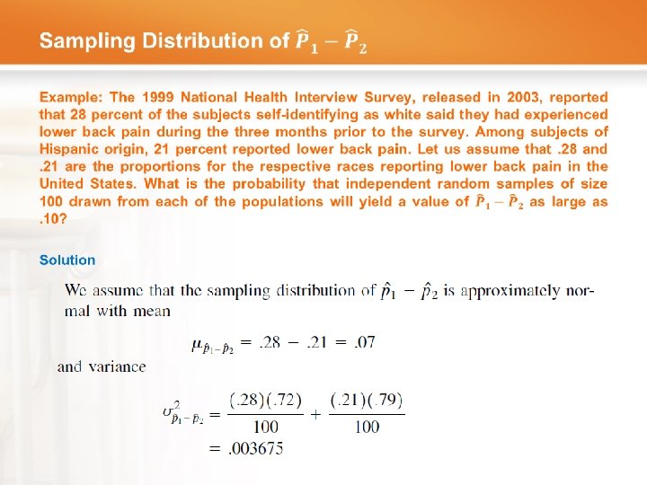
Consulting the table, we find that the area under the standard normal curve that lies to the right of z =. 49 is 1 -. 6879 =. 3121. The probability of observing a difference as large as. 10 is, then, . 3121.

Example: In the 1999 National Health Interview Survey, researchers found that among U. S. adults ages 75 or older, 34 percent had lost all their natural teeth and for U. S. adults ages 65– 74, 26 percent had lost all their natural teeth. Assume that these proportions are the parameters for the United States in those age groups. If a random sample of 250 adults ages 65– 74 and an independent random sample of 200 adults ages 45– 64 years old are drawn from these populations, find the probability that the difference in percent of total natural teeth loss is less than 5 percent between the two populations. Solution Continue on next slide…

Consulting the Table, we find that the area to the left of z = -. 70 is. 2420.

Thank You !!!