Probability and Statistics with Reliability Queuing and Computer

Probability and Statistics with Reliability, Queuing and Computer Science Applications: Chapter 6 on Stochastic Processes Kishor S. Trivedi Visiting Professor Dept. of Computer Science and Engineering Indian Institute of Technology, Kanpur

What is a Stochastic Process? n n Stochastic Process: is a family of random variables {X(t) | t ε T} (T is an index set; it may be discrete or continuous) Values assumed by X(t) are called states. State space (I): set of all possible states Sometimes called a random process or a chance process

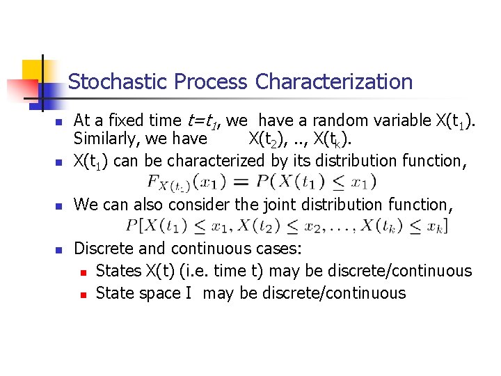
Stochastic Process Characterization n At a fixed time t=t 1, we have a random variable X(t 1). Similarly, we have X(t 2), . . , X(tk). X(t 1) can be characterized by its distribution function, n We can also consider the joint distribution function, n n Discrete and continuous cases: n States X(t) (i. e. time t) may be discrete/continuous n State space I may be discrete/continuous

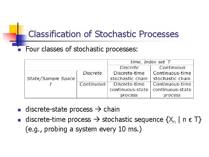
Classification of Stochastic Processes n n n Four classes of stochastic processes: discrete-state process chain discrete-time process stochastic sequence {Xn | n є T} (e. g. , probing a system every 10 ms. )

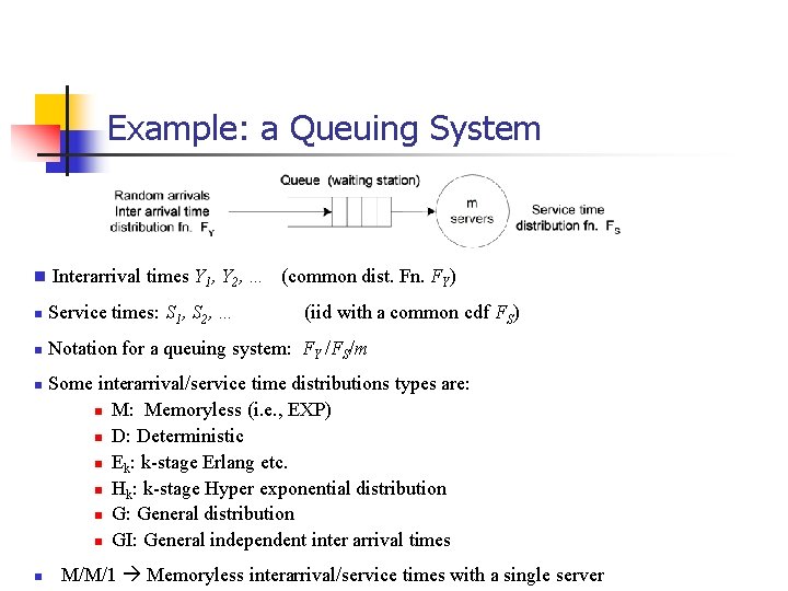
Example: a Queuing System n Interarrival times Y 1, Y 2, … (common dist. Fn. FY) n Service times: S 1, S 2, … n Notation for a queuing system: FY /FS/m n n (iid with a common cdf FS) Some interarrival/service time distributions types are: n M: Memoryless (i. e. , EXP) n D: Deterministic n Ek: k-stage Erlang etc. n Hk: k-stage Hyper exponential distribution n G: General distribution n GI: General independent inter arrival times M/M/1 Memoryless interarrival/service times with a single server

Discrete/Continuous Stochastic Processes Nk: Number of jobs waiting in the system at the time of kth job’s departure Stochastic process {Nk| k=1, 2, …}: n Discrete time, discrete state Nk Discrete n Discrete k

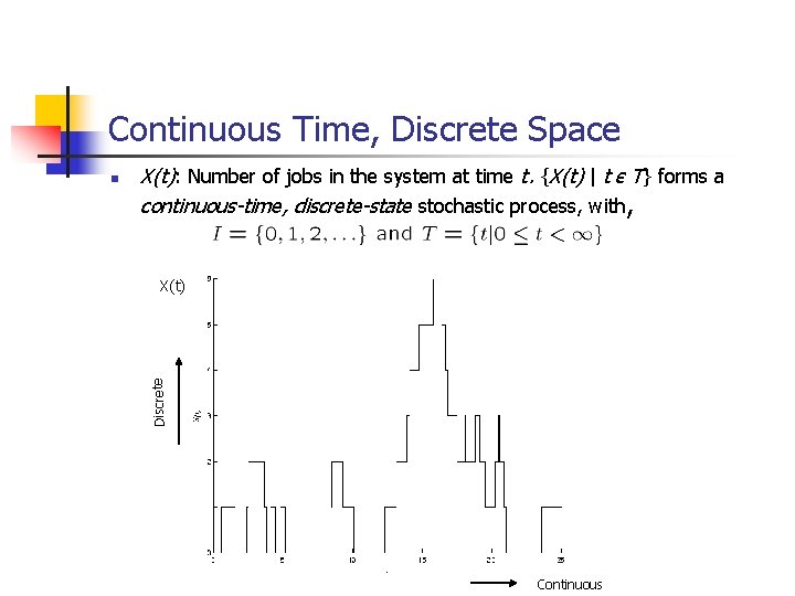
Continuous Time, Discrete Space X(t): Number of jobs in the system at time t. {X(t) | t є T} forms a continuous-time, discrete-state stochastic process, with, X(t) Discrete n Continuous

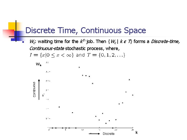
Discrete Time, Continuous Space Wk: waiting time for the kth job. Then {Wk | k є T} forms a Discrete-time, Continuous-state stochastic process, where, Wk Continuous n Discrete k

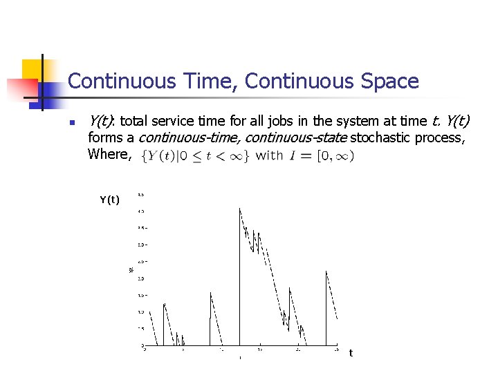
Continuous Time, Continuous Space n Y(t): total service time for all jobs in the system at time t. Y(t) forms a continuous-time, continuous-state stochastic process, Where, Y(t) t

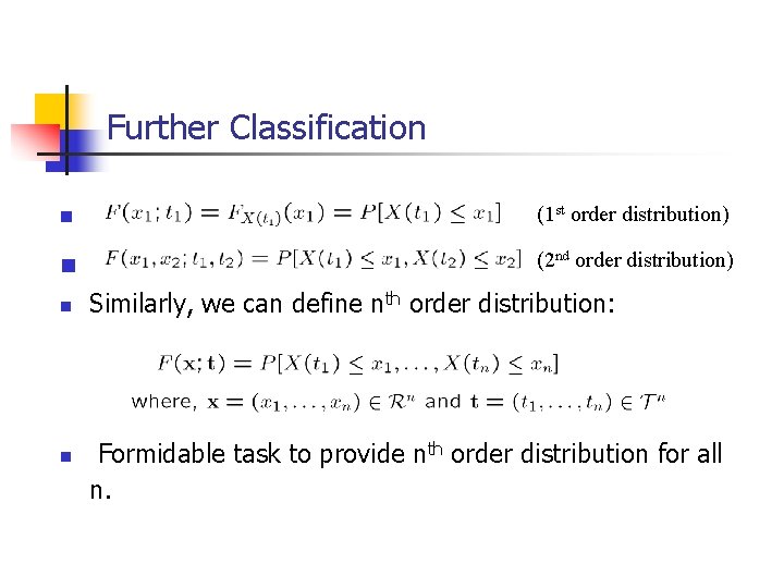
Further Classification n (1 st order distribution) n (2 nd order distribution) n n Similarly, we can define nth order distribution: Formidable task to provide nth order distribution for all n.

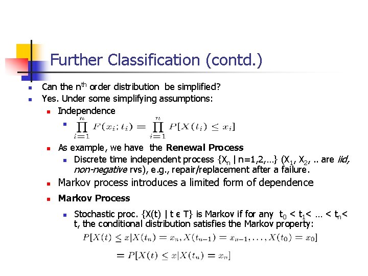
Further Classification (contd. ) n n Can the nth order distribution be simplified? Yes. Under some simplifying assumptions: n Independence n n As example, we have the Renewal Process n Discrete time independent process {Xn | n=1, 2, …} (X 1, X 2, . . are iid, non-negative rvs), e. g. , repair/replacement after a failure. n Markov process introduces a limited form of dependence n Markov Process n Stochastic proc. {X(t) | t є T} is Markov if for any t 0 < t 1< … < tn< t, the conditional distribution satisfies the Markov property:

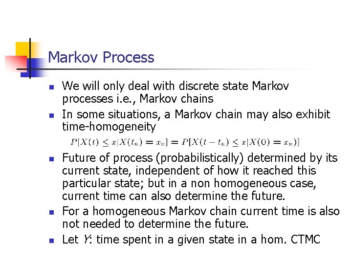
Markov Process n n n We will only deal with discrete state Markov processes i. e. , Markov chains In some situations, a Markov chain may also exhibit time-homogeneity Future of process (probabilistically) determined by its current state, independent of how it reached this particular state; but in a non homogeneous case, current time can also determine the future. For a homogeneous Markov chain current time is also not needed to determine the future. Let Y: time spent in a given state in a hom. CTMC

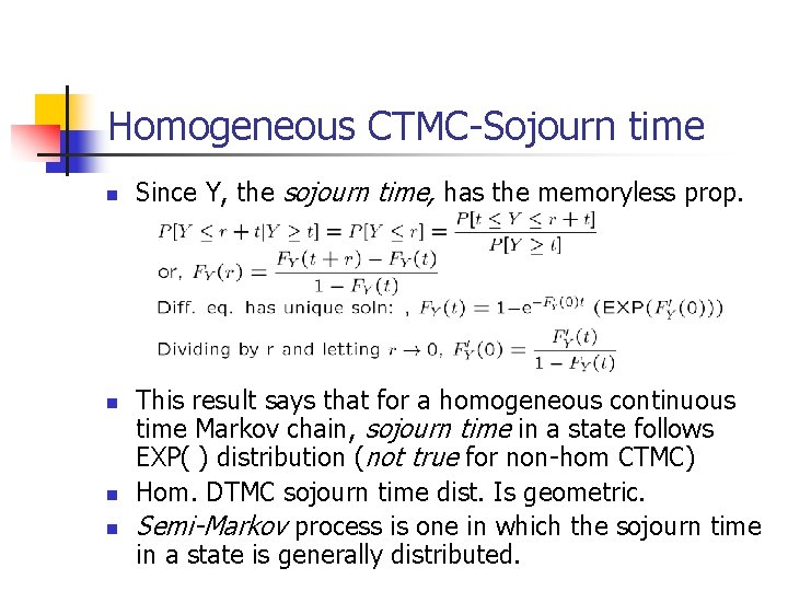
Homogeneous CTMC-Sojourn time n n Since Y, the sojourn time, has the memoryless prop. This result says that for a homogeneous continuous time Markov chain, sojourn time in a state follows EXP( ) distribution (not true for non-hom CTMC) Hom. DTMC sojourn time dist. Is geometric. Semi-Markov process is one in which the sojourn time in a state is generally distributed.

Bernoulli Process n n n A sequence of iid Bernoulli rvs, {Yi | i=1, 2, 3, . . }, Yi =1 or 0 {Yi} forms a Bernoulli Process, an example of a renewal process. Define another stochastic process , {Sn | n=1, 2, 3, . . }, where Sn = Y 1 + Y 2 +…+ Yn (i. e. Sn : sequence of partial sums) n Sn = Sn-1+ Yn (recursive form) n P[Sn = k | Sn-1= k] = P[Yn = 0] = (1 -p) and, n P[Sn = k | Sn-1= k-1] = P[Yn = 1] = p n {Sn |n=1, 2, 3, . . }, forms a Binomial process, an example of a homogeneous DTMC

Renewal Counting Process n n Renewal counting process: # of renewals (repairs, replacements, arrivals) by time t: a continuous time process: If time interval between two renewals follows EXP distribution, then Poisson Process

Note: For a fixed t, N(t) is a random variable (in this case a discrete random variable known as the Poisson random variable) n. The family {N(t), t 0} is a stochastic process, in this case, the homogeneous Poisson process n{N(t), t 0} is a homogeneous CTMC as well n

Poisson Process n n n A continuous time, discrete state process. N(t): no. of events occurring in time (0, t]. Events may be, 1. # of packets arriving at a router port 2. # of incoming telephone calls at a switch 3. # of jobs arriving at file/compute server 4. Number of component failures Events occurs successively and that intervals between these successive events are iid rvs, each following EXP( ) 5. 6. λ: arrival rate (1/ λ: average time between arrivals) λ: failure rate (1/ λ: average time between failures)

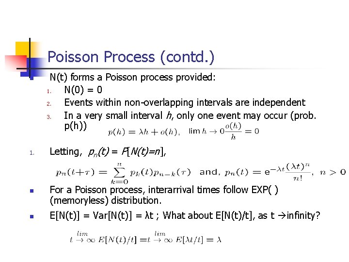
Poisson Process (contd. ) n 1. n n N(t) forms a Poisson process provided: 1. N(0) = 0 2. Events within non-overlapping intervals are independent 3. In a very small interval h, only one event may occur (prob. p(h)) Letting, pn(t) = P[N(t)=n], For a Poisson process, interarrival times follow EXP( ) (memoryless) distribution. E[N(t)] = Var[N(t)] = λt ; What about E[N(t)/t], as t infinity?

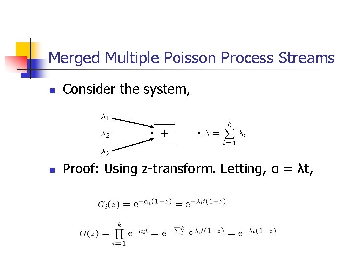
Merged Multiple Poisson Process Streams n Consider the system, + n Proof: Using z-transform. Letting, α = λt,

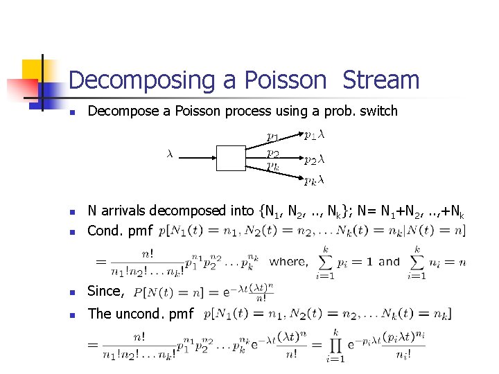
Decomposing a Poisson Stream n Decompose a Poisson process using a prob. switch n N arrivals decomposed into {N 1, N 2, . . , Nk}; N= N 1+N 2, . . , +Nk Cond. pmf n Since, n The uncond. pmf n

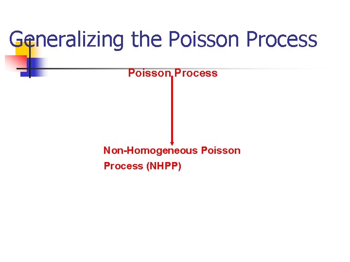
Generalizing the Poisson Process Non-Homogeneous Poisson Process (NHPP)

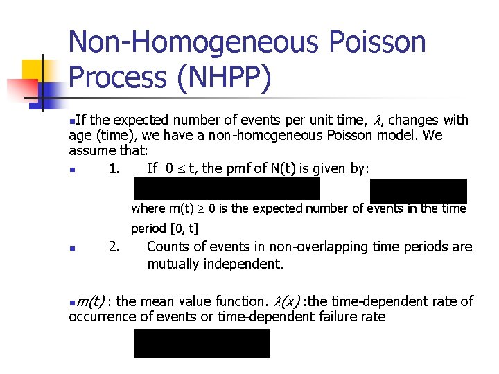
Non-Homogeneous Poisson Process (NHPP) If the expected number of events per unit time, l, changes with age (time), we have a non-homogeneous Poisson model. We assume that: n 1. If 0 t, the pmf of N(t) is given by: n where m(t) 0 is the expected number of events in the time period [0, t] n n 2. Counts of events in non-overlapping time periods are mutually independent. m(t) : the mean value function. l(x) : the time-dependent rate of occurrence of events or time-dependent failure rate

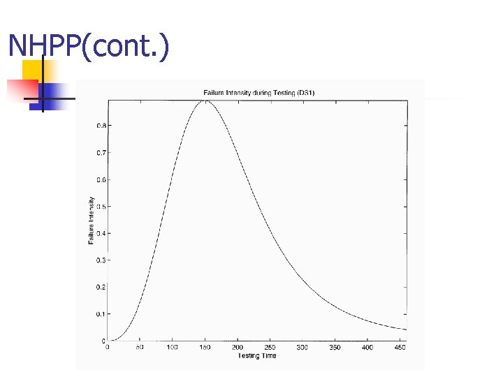
NHPP(cont. )

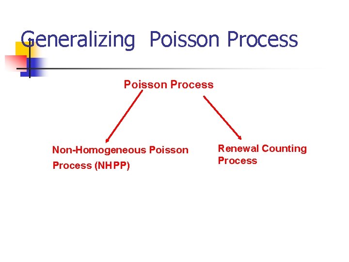
Generalizing Poisson Process Non-Homogeneous Poisson Process (NHPP) Renewal Counting Process

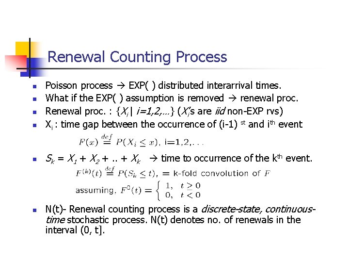
Renewal Counting Process n Poisson process EXP( ) distributed interarrival times. What if the EXP( ) assumption is removed renewal proc. Renewal proc. : {Xi | i=1, 2, …} (Xi’s are iid non-EXP rvs) Xi : time gap between the occurrence of (i-1) st and ith event n Sk = X 1 + X 2 +. . + Xk time to occurrence of the kth event. n n N(t)- Renewal counting process is a discrete-state, continuoustime stochastic process. N(t) denotes no. of renewals in the interval (0, t].

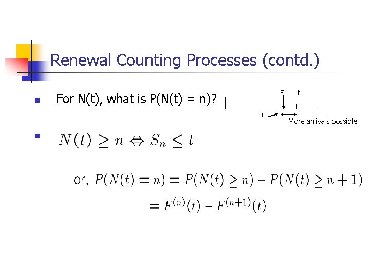
Renewal Counting Processes (contd. ) n Sn For N(t), what is P(N(t) = n)? tn n t More arrivals possible

Renewal Counting Process Expectation n Let, m(t) = E[N(t)]. Then, m(t) = mean no. of arrivals in time (0, t]. m(t) is called the renewal function.

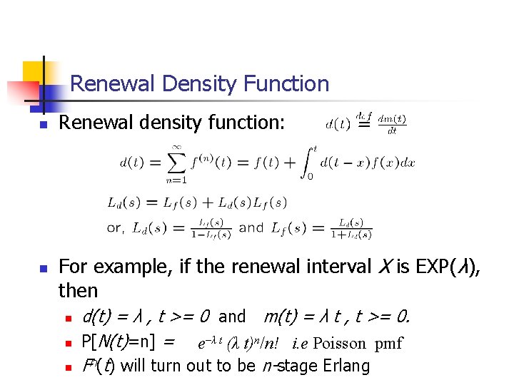
Renewal Density Function n n Renewal density function: For example, if the renewal interval X is EXP(λ), then n d(t) = λ , t >= 0 and m(t) = λ t , t >= 0. P[N(t)=n] = e–λ t (λ t)n/n! i. e Poisson pmf Fn(t) will turn out to be n-stage Erlang

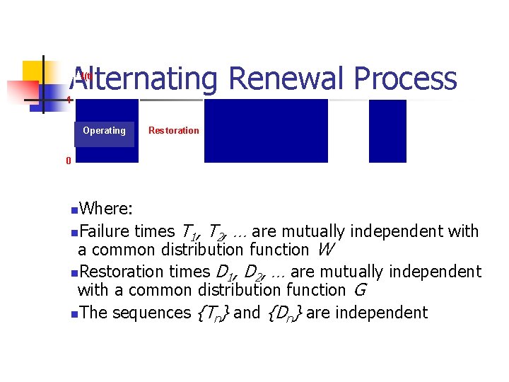
Alternating Renewal Process I(t) 1 Operating Restoration 0 Time Where: n. Failure times T 1, T 2, … are mutually independent with a common distribution function W n. Restoration times D 1, D 2, … are mutually independent with a common distribution function G n. The sequences {Tn} and {Dn} are independent n

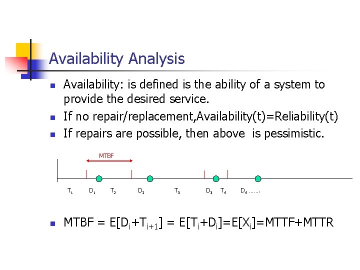
Availability Analysis n n n Availability: is defined is the ability of a system to provide the desired service. If no repair/replacement, Availability(t)=Reliability(t) If repairs are possible, then above is pessimistic. MTBF T 1 n D 1 T 2 D 2 T 3 D 3 T 4 D 4 ……. MTBF = E[Di+Ti+1] = E[Ti+Di]=E[Xi]=MTTF+MTTR

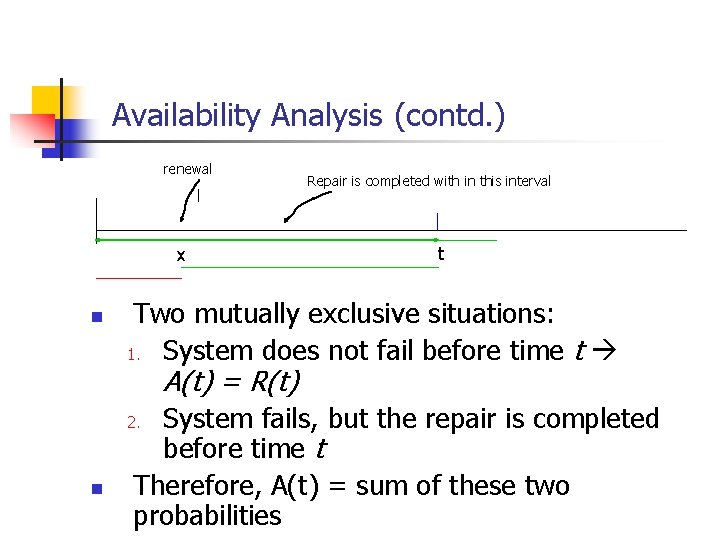
Availability Analysis (contd. ) renewal x n Repair is completed with in this interval t Two mutually exclusive situations: 1. System does not fail before time t A(t) = R(t) System fails, but the repair is completed before time t Therefore, A(t) = sum of these two probabilities 2. n

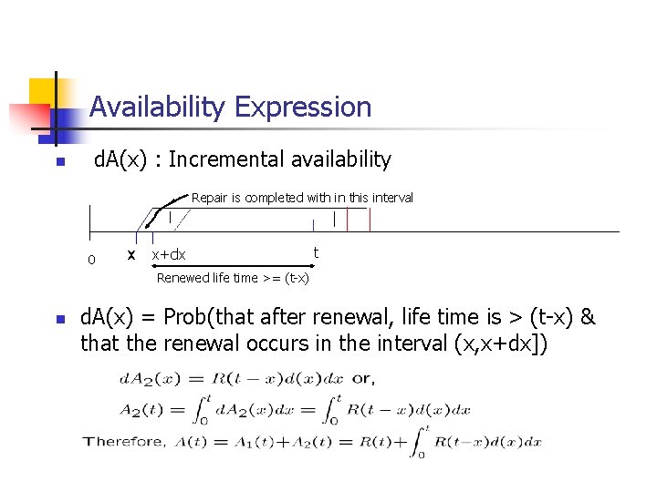
Availability Expression n d. A(x) : Incremental availability Repair is completed with in this interval 0 x x+dx t Renewed life time >= (t-x) n d. A(x) = Prob(that after renewal, life time is > (t-x) & that the renewal occurs in the interval (x, x+dx])

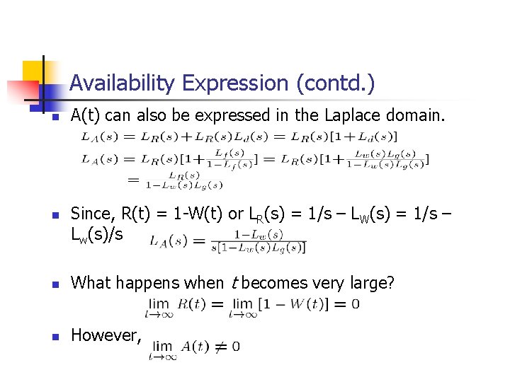
Availability Expression (contd. ) n n A(t) can also be expressed in the Laplace domain. Since, R(t) = 1 -W(t) or LR(s) = 1/s – LW(s) = 1/s – Lw(s)/s n What happens when t becomes very large? n However,

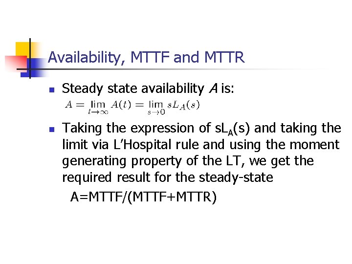
Availability, MTTF and MTTR n n Steady state availability A is: Taking the expression of s. LA(s) and taking the limit via L’Hospital rule and using the moment generating property of the LT, we get the required result for the steady-state A=MTTF/(MTTF+MTTR)

Availability Example n Assuming EXP( ) density fn for g(t) and w(t)

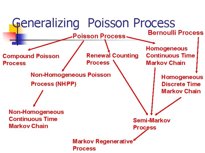
Generalizing Poisson Process Bernoulli Process Poisson Process Renewal Counting Process Compound Poisson Process Non-Homogeneous Poisson Process (NHPP) Non-Homogeneous Continuous Time Markov Chain Homogeneous Discrete Time Markov Chain Semi-Markov Process Markov Regenerative Process