Probability and Statistics Honors Chapter 2 Modeling Distributions

Describing Location in a Distribution • In order to describe individuals within a distribution, we may wish to look at their placement relative to the other subjects. • To measure such a relative position, we will calculate the subject’s percentile. • The pth percentile of a distribution is the value in the distribution with p percent of the data less than it. • It is important that the data be in numerical order before this calculation is done. 2

Cumulative Relative Frequency Graphs • REMEMBER: The relative frequency of something is the percent of items in that class out of the total. • Cumulative – the total of everything up to that point. • Cumulative Relative Frequency is the sum of all of the percentages up to the given point. • Since the values are cumulative, they will be constantly increasing until they get to 100%. 3

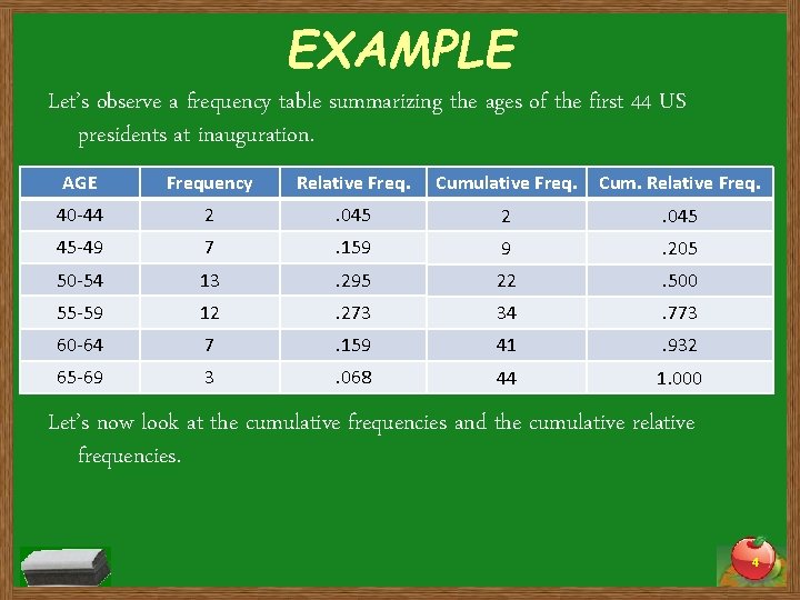
EXAMPLE Let’s observe a frequency table summarizing the ages of the first 44 US presidents at inauguration. AGE Frequency Relative Freq. Cumulative Freq. Cum. Relative Freq. 40 -44 2 . 045 45 -49 7 . 159 9 . 205 50 -54 13 . 295 22 . 500 55 -59 12 . 273 34 . 773 60 -64 7 . 159 41 . 932 65 -69 let’s look at 3 the relative frequencies. 068 1. 000 Now for each 44 class. Let’s now look at the cumulative frequencies and the cumulative relative frequencies. 4

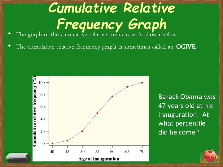
Cumulative Relative Frequency Graph • The graph of the cumulative relative frequencies is shown below. • The cumulative relative frequency graph is sometimes called an OGIVE. Barack Obama was 47 years old at his inauguration. At what percentile did he come? 5

Applying the Concepts • Complete the “Check Your Understanding” questions on pg. 89.

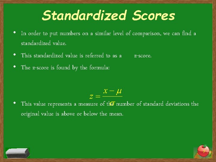
Standardized Scores • In order to put numbers on a similar level of comparison, we can find a standardized value. • This standardized value is referred to as a z-score. • The z-score is found by the formula: • This value represents a measure of the number of standard deviations the original value is above or below the mean. 7

EXAMPLE • Jenny scored an 86 on her statistics test. She was satisfied with this, but was upset by a score of 82 on her chemistry test. • Jenny later learned that both sets of tests had symmetric distributions. • The statistics test had a mean score of 80 with a standard deviation of 6. 07. • The chemistry test had a mean score of 76, with a standard deviation of 4. • In comparison to the other students taking the tests, on which test did Jenny perform better? 8

Applying the Concepts • Complete the “Check Your Understanding” questions on pg. 91.

HOMEWORK Complete the assignment listed in the packet. This assignment will be due at the beginning of the next class session. 10

Density Curves • • • A density curve is a curve that is always on or above the horizontal axis. The area under a density curve is always equal to 1. It is used to describe the overall pattern of a distribution. The median divides the area under the curve in half. The mean can be considered the “balance point” of the curve.

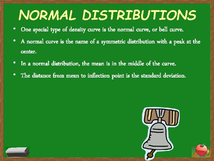
NORMAL DISTRIBUTIONS • One special type of density curve is the normal curve, or bell curve. • A normal curve is the name of a symmetric distribution with a peak at the center. • In a normal distribution, the mean is in the middle of the curve. • The distance from mean to inflection point is the standard deviation.

The 68 -95 -99. 7 Rule • In a normal distribution, we are looking at an entire population. • Because of this, we call our mean μ and we call our standard deviation σ. • In a normal distribution, we can use the 68 -95 -99. 7 Rule to estimate the amount of data in an area under the curve based on its μ and σ.

68 -95 -99. 7 Continued • Based on this rule, an estimated 68% of the data will come within one standard deviation of the mean. • Within two standard deviations of the mean, approximately 95% of the data will fall. • An estimated 99. 7% will fall within three standard deviations of the mean. • This means that only 0. 3% of data is more than 3σ away from μ.

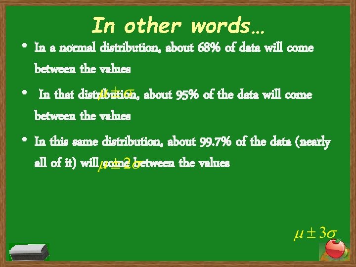
In other words… • In a normal distribution, about 68% of data will come between the values • In that distribution, about 95% of the data will come between the values • In this same distribution, about 99. 7% of the data (nearly all of it) will come between the values

EXAMPLE The height of women aged 18 -24 is approximately normal with a mean μ = 64. 5 inches and a standard deviation σ = 2. 5. What two heights could we expect 68% of women to fall between? What two heights would 95% of women come between? What percent of women are taller than 6 feet tall?

EXAMPLE 2 • The distribution of SAT-Math scores is approximately N(500, 100). • What percent of students score between 400 and 600? • Between what two scores would 95% of the students taking the test score? • What percent of students score above 700? 17

VIDEO #7 Decisions Through Data Normal Curves 18

HOMEWORK Complete pg. 108(#27 – 38) pg. 131(#41 – 46) and video #7 problems. This assignment will be due for completion at the start of the next session of class.

• Normal Distribution Calculations We can use the z-score of a value to determine the percentage of data that is less than that value. • To do this, we can use the z-score table located in the book. • The table is located in back of your book (Table A). • It can be used to find the percent of data to the left of any zscore.

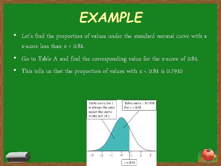
EXAMPLE • Let’s find the proportion of values under the standard normal curve with a z-score less than z = 0. 81. • Go to Table A and find the corresponding value for the z-score of 0. 81. • This tells us that the proportion of values with z < 0. 81 is 0. 7910 21

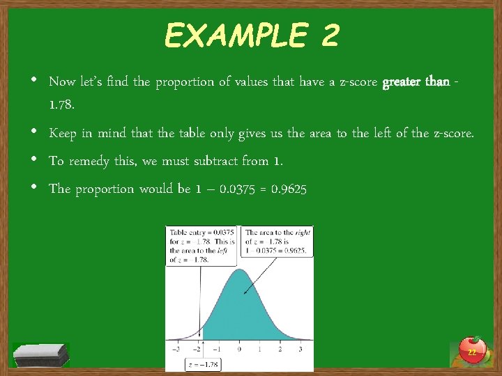
EXAMPLE 2 • Now let’s find the proportion of values that have a z-score greater than 1. 78. • Keep in mind that the table only gives us the area to the left of the z-score. • To remedy this, we must subtract from 1. • The proportion would be 1 – 0. 0375 = 0. 9625 22

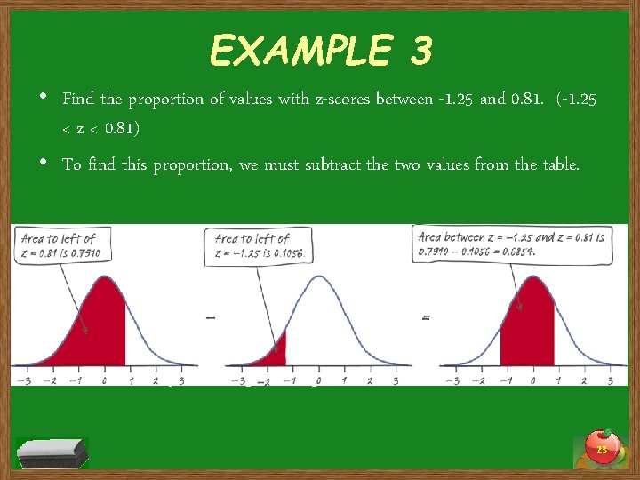
EXAMPLE 3 • Find the proportion of values with z-scores between -1. 25 and 0. 81. (-1. 25 < z < 0. 81) • To find this proportion, we must subtract the two values from the table. • The area is 0. 7910 – 0. 1056 = 0. 6854. 23

Applying the Concepts • Complete the “Check Your Understanding” questions on pg. 119.

Normal Distribution Calculations • Often, we will deal with a normal distribution of numbers with a mean different than N(0, 1). • In these cases, we must standardize the value before we can use Table A. EXAMPLE When Tiger Woods hits his driver, the distance the ball travels follows a normal distribution with mean of 304 yds. and a standard deviation of 8 yds. What percent of his drives travel at least 290? 25

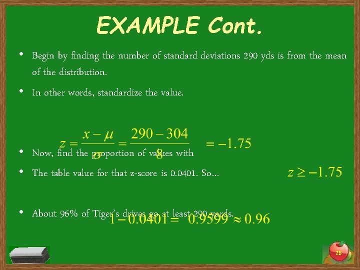
EXAMPLE Cont. • Begin by finding the number of standard deviations 290 yds is from the mean of the distribution. • In other words, standardize the value. • Now, find the proportion of values with • The table value for that z-score is 0. 0401. So… • About 96% of Tiger’s drives go at least 290 yards. 26

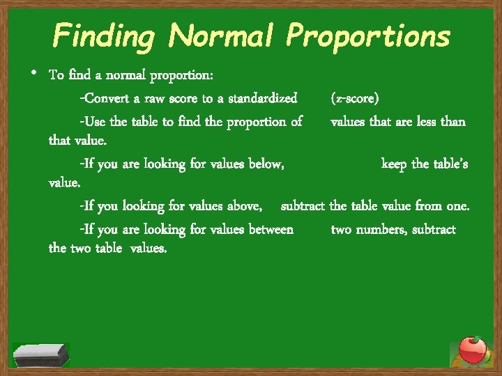
Finding Normal Proportions • To find a normal proportion: -Convert a raw score to a standardized (z-score) -Use the table to find the proportion of values that are less than that value. -If you are looking for values below, keep the table’s value. -If you looking for values above, subtract the table value from one. -If you are looking for values between two numbers, subtract the two table values.

Applying the Concepts • Complete the “Check Your Understanding” questions on pg. 124.

HOMEWORK Complete pg. 131 (#47 – 58). This assignment will be due for completion at the start of the next session of class.