Probability and Statistics for Ensemble Forecasting Tom Hamill

Probability and Statistics for Ensemble Forecasting Tom Hamill (NOAA/ESRL, Boulder) and Jim Hansen (Naval Research Lab, Monterey) (borrows heavily from Dan Wilks’ Statistical Methods in the Atmospheric Sciences text)

Probability and statistics: (1) inherently confusing, or (2) a formal way of bamboozling and waffling? “Doctors say that Nordberg has a 50/50 chance of living, though there's only a 10 percent chance of that. ”

Probability and statistics • Probability: a formalism for expressing uncertainty quantitatively. • Statistics: the science pertaining to the collection, analysis, interpretation or explanation, and presentation of data. • Goal: get you comfortable with the terminology the other instructors will use.

Part 1: Probability Weather is uncertain, so we use the language of uncertainty photo courtesy of Lenny Smith, Oxford U. and London School of Economics

Probability religions • The Frequentists: probability is the long-run expected frequency of occurrence. • The Bayesians: probability is a degree of believability. “A Frequentist is a person whose long-run ambition is to be wrong 5% of the time. ” “A Bayesian is one who, vaguely expecting a horse, and catching a glimpse of a donkey, strongly believes he has seen a mule. ” Should this matter to you? Luckily, no…we all worship the same mathematical deity.

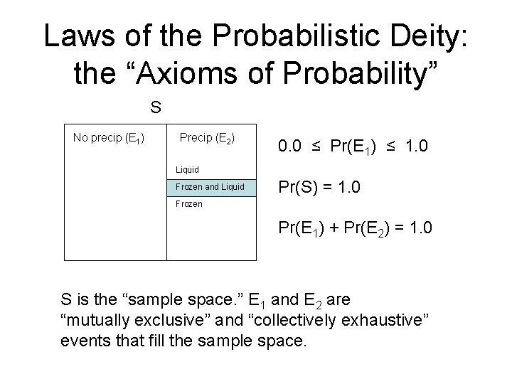
Laws of the Probabilistic Deity: the “Axioms of Probability” S No precip (E 1) Precip (E 2) 0. 0 ≤ Pr(E 1) ≤ 1. 0 Liquid Frozen and Liquid Pr(S) = 1. 0 Frozen Pr(E 1) + Pr(E 2) = 1. 0 S is the “sample space. ” E 1 and E 2 are “mutually exclusive” and “collectively exhaustive” events that fill the sample space.

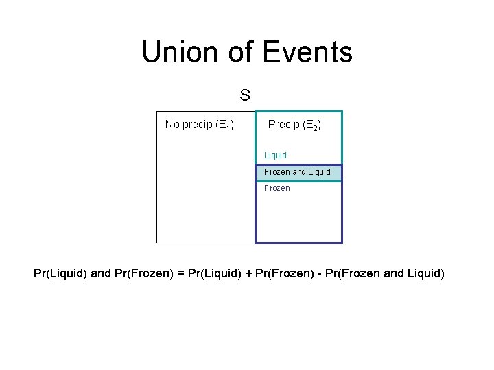
Union of Events S No precip (E 1) Precip (E 2) Liquid Frozen and Liquid Frozen Pr(Liquid) and Pr(Frozen) = Pr(Liquid) + Pr(Frozen) - Pr(Frozen and Liquid)

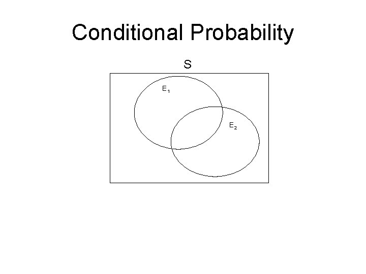
Conditional Probability S E 1 E 2

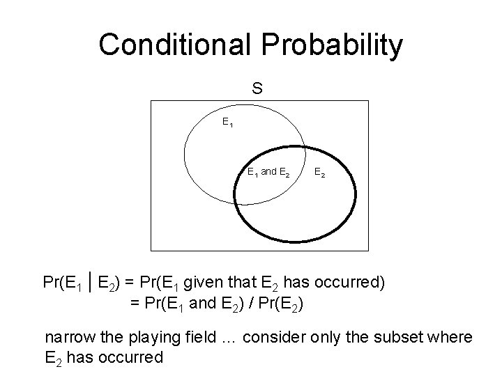
Conditional Probability S E 1 and E 2 Pr(E 1 | E 2) = Pr(E 1 given that E 2 has occurred) = Pr(E 1 and E 2) / Pr(E 2) narrow the playing field … consider only the subset where E 2 has occurred

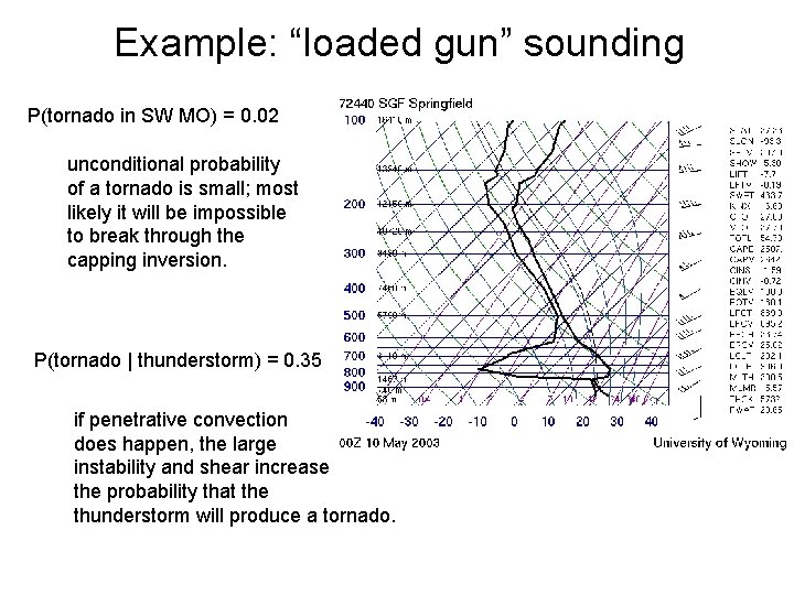
Example: “loaded gun” sounding P(tornado in SW MO) = 0. 02 unconditional probability of a tornado is small; most likely it will be impossible to break through the capping inversion. P(tornado | thunderstorm) = 0. 35 if penetrative convection does happen, the large instability and shear increase the probability that the thunderstorm will produce a tornado.

Independence • E 1 and E 2 are independent if and only if Pr (E 1 and E 2) = Pr (E 1) x Pr (E 2) Probability of two sixes = 1/6 x 1/6 = 1/36

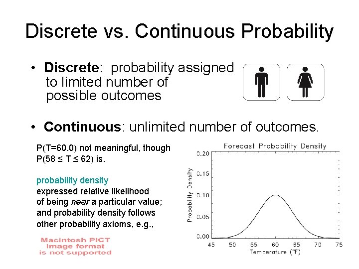
Discrete vs. Continuous Probability • Discrete: probability assigned to limited number of possible outcomes • Continuous: unlimited number of outcomes. P(T=60. 0) not meaningful, though P(58 ≤ T ≤ 62) is. probability density expressed relative likelihood of being near a particular value; and probability density follows other probability axioms, e. g. ,

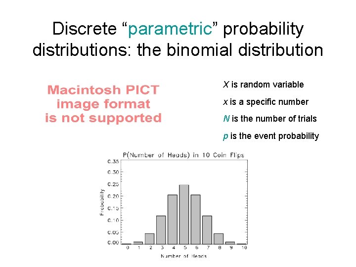
Discrete “parametric” probability distributions: the binomial distribution X is random variable x is a specific number N is the number of trials p is the event probability

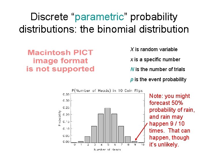
Discrete “parametric” probability distributions: the binomial distribution X is random variable x is a specific number N is the number of trials p is the event probability Note: you might forecast 50% probability of rain, and rain may happen 9 / 10 times. That can happen, though it’s unlikely.

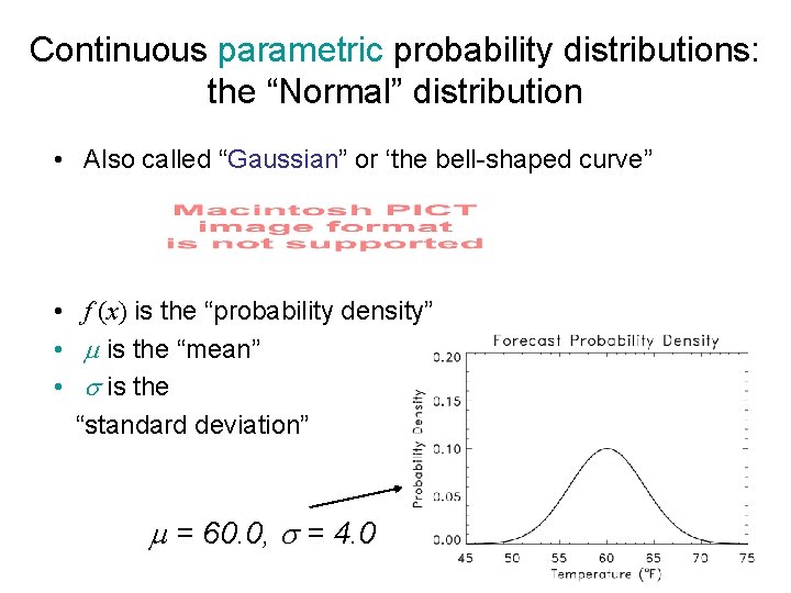
Continuous parametric probability distributions: the “Normal” distribution • Also called “Gaussian” or ‘the bell-shaped curve” • f (x) is the “probability density” • is the “mean” • is the “standard deviation” = 60. 0, = 4. 0

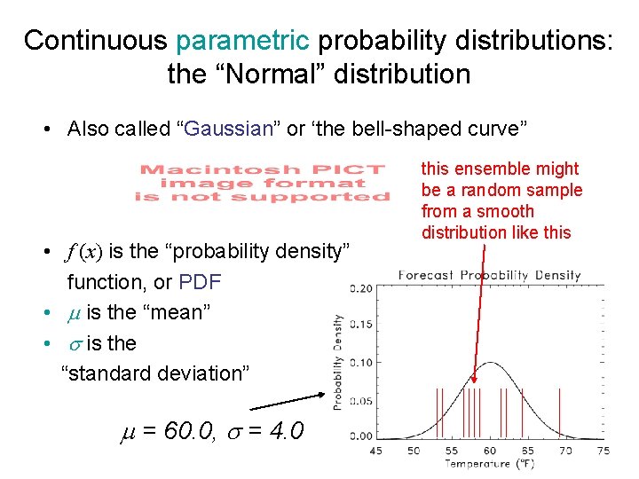
Continuous parametric probability distributions: the “Normal” distribution • Also called “Gaussian” or ‘the bell-shaped curve” • f (x) is the “probability density” function, or PDF • is the “mean” • is the “standard deviation” = 60. 0, = 4. 0 this ensemble might be a random sample from a smooth distribution like this

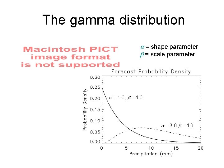
The gamma distribution = shape parameter = scale parameter = 1. 0, = 4. 0 = 3. 0 = 4. 0

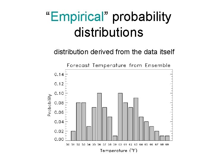
“Empirical” probability distributions distribution derived from the data itself

Statistics Definition: “the science pertaining to the collection, analysis, interpretation or explanation, and presentation of data. ”

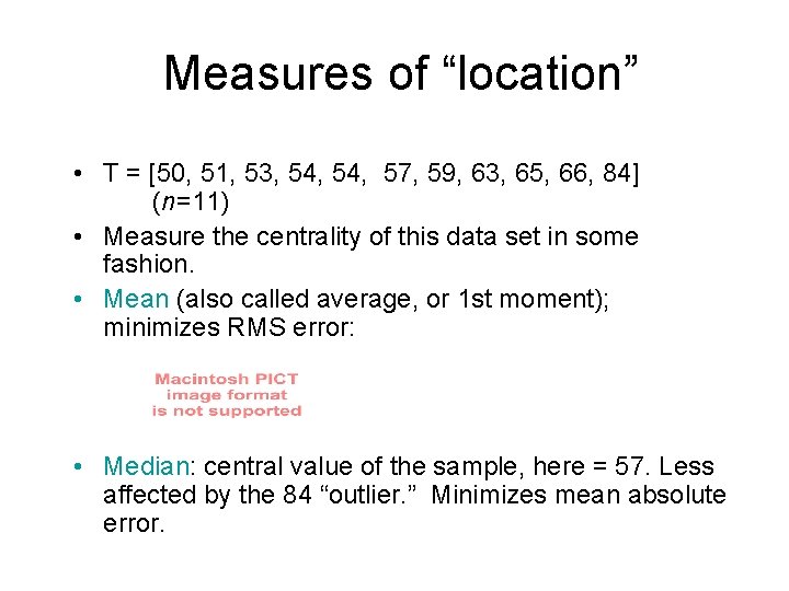
Measures of “location” • T = [50, 51, 53, 54, 57, 59, 63, 65, 66, 84] (n=11) • Measure the centrality of this data set in some fashion. • Mean (also called average, or 1 st moment); minimizes RMS error: • Median: central value of the sample, here = 57. Less affected by the 84 “outlier. ” Minimizes mean absolute error.

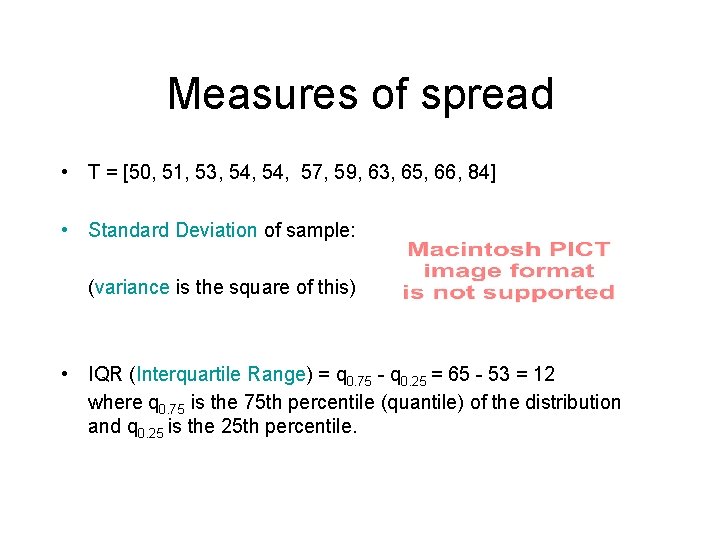
Measures of spread • T = [50, 51, 53, 54, 57, 59, 63, 65, 66, 84] • Standard Deviation of sample: (variance is the square of this) • IQR (Interquartile Range) = q 0. 75 - q 0. 25 = 65 - 53 = 12 where q 0. 75 is the 75 th percentile (quantile) of the distribution and q 0. 25 is the 25 th percentile.

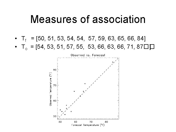
Measures of association • Tf = [50, 51, 53, 54, 57, 59, 63, 65, 66, 84] • To = [54, 53, 51, 57, 55, 53, 66, 63, 66, 71, 87�� ]

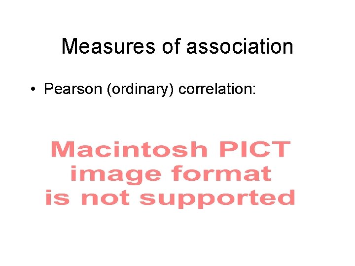
Measures of association • Pearson (ordinary) correlation:

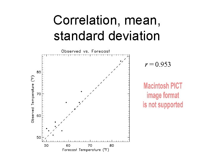
Correlation, mean, standard deviation r = 0. 953

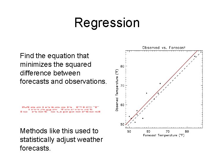
Regression Find the equation that minimizes the squared difference between forecasts and observations. Methods like this used to statistically adjust weather forecasts.

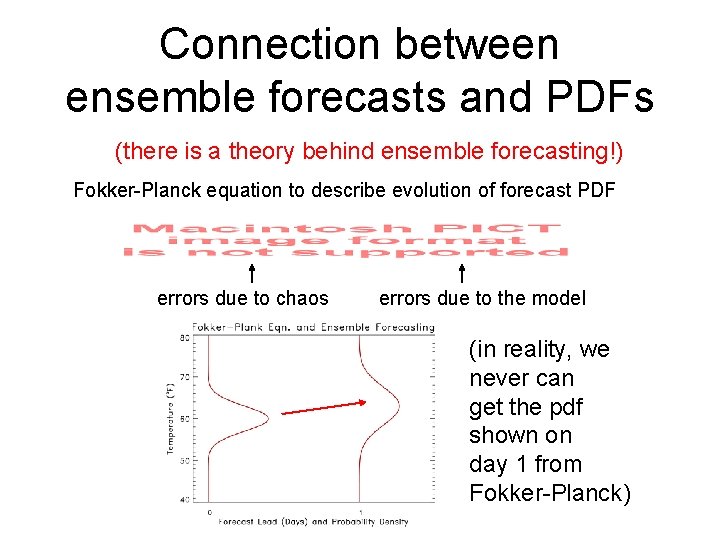
Connection between ensemble forecasts and PDFs (there is a theory behind ensemble forecasting!) Fokker-Planck equation to describe evolution of forecast PDF errors due to chaos errors due to the model (in reality, we never can get the pdf shown on day 1 from Fokker-Planck)

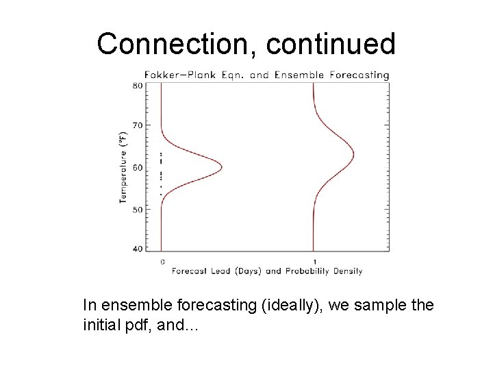
Connection, continued In ensemble forecasting (ideally), we sample the initial pdf, and…

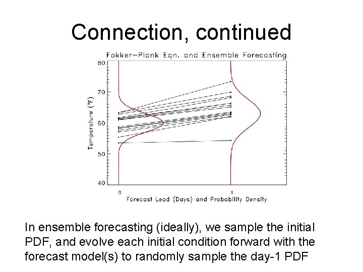
Connection, continued In ensemble forecasting (ideally), we sample the initial PDF, and evolve each initial condition forward with the forecast model(s) to randomly sample the day-1 PDF

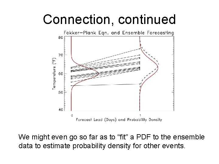
Connection, continued We might even go so far as to “fit” a PDF to the ensemble data to estimate probability density for other events.

Questions?

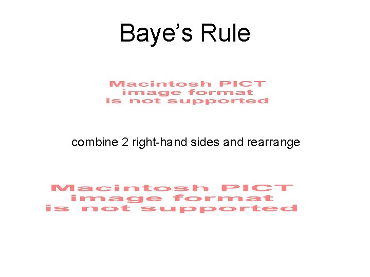
Baye’s Rule combine 2 right-hand sides and rearrange

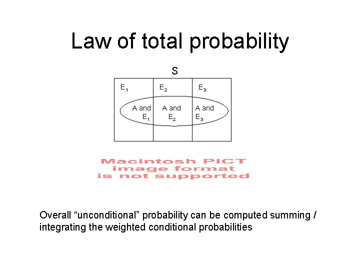
Law of total probability S E 1 E 2 A and E 1 A and E 2 E 3 A and E 3 Overall “unconditional” probability can be computed summing / integrating the weighted conditional probabilities

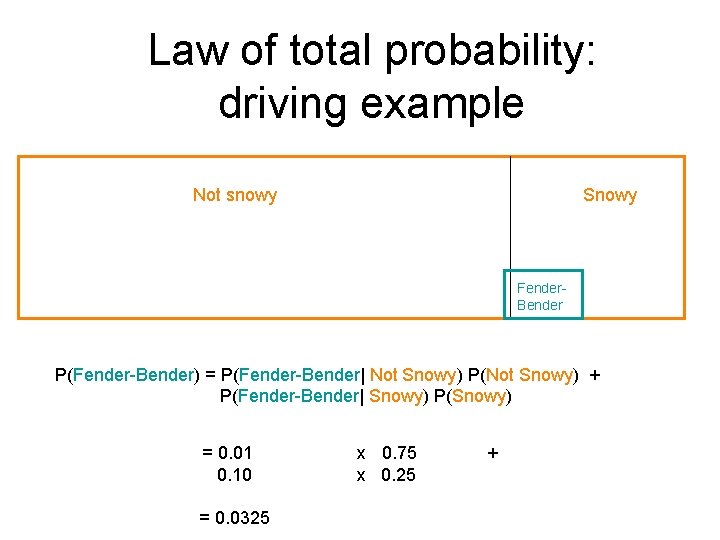
Law of total probability: driving example Not snowy Snowy Fender. Bender P(Fender-Bender) = P(Fender-Bender| Not Snowy) P(Not Snowy) + P(Fender-Bender| Snowy) P(Snowy) = 0. 01 0. 10 = 0. 0325 x 0. 75 x 0. 25 +

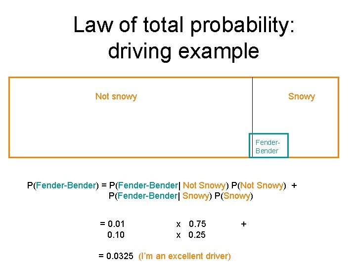
Law of total probability: driving example Not snowy Snowy Fender. Bender P(Fender-Bender) = P(Fender-Bender| Not Snowy) P(Not Snowy) + P(Fender-Bender| Snowy) P(Snowy) = 0. 01 0. 10 x 0. 75 x 0. 25 = 0. 0325 (I’m an excellent driver) +

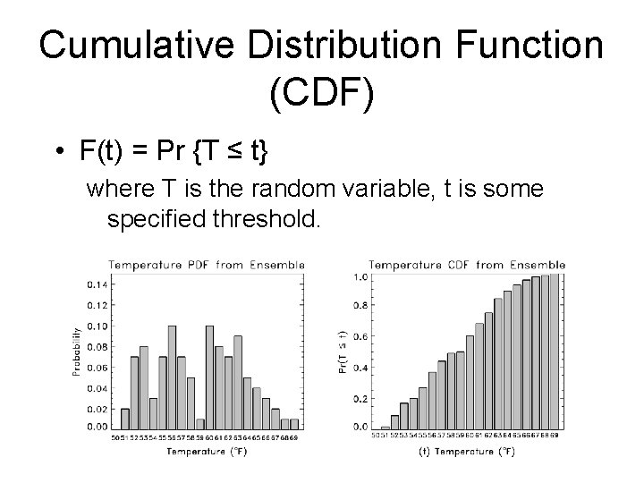
Cumulative Distribution Function (CDF) • F(t) = Pr {T ≤ t} where T is the random variable, t is some specified threshold.