Probability and Statistics for Computer Scientists Third Edition

Probability and Statistics for Computer Scientists Third Edition, By Michael Baron Chapter 8: Introduction to Statistics CIS 2033. Computational Probability and Statistics Pei Wang

Statistics: the analysis and interpretation of data, where the set of observations is called a “dataset” or “sample” Assumptions: • The observations are the values of random variables of the same type • The sample represents the population from which it is selected

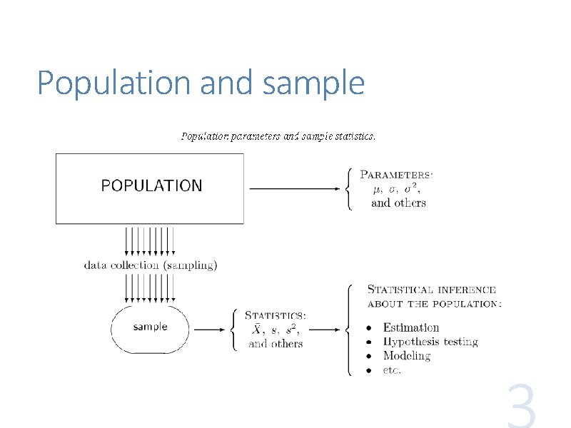
Population and sample

Topics in statistics From data to model (the reverse of simulation), or from sample to population • to summarize and visualize the data • to approximate the (p, f, or F) function that specifies the model • to estimate a parameter of a model • to estimate a population feature using a sample statistic

Sampling What is the right way to do sampling? Simple random sampling: data are collected from the entire population independently of each other, all being equally likely to be selected This process reduces the bias in the sample x 1, …, xn, which is taken to be values of iid (independent, identically distributed) random variables X 1, …, Xn

Parameter estimation A dataset is often modeled as a realization of a random sample from a probability distribution determined by one or more parameters Let t = h(x 1, . . . , xn) be an estimate of a parameter based on the dataset x 1, . . . , xn only Then t is a realization of the random variable T = h(X 1, . . . , Xn), which is called an estimator

Bias and consistency An estimator T (or θ-hat, ) is called an unbiased estimator for the parameter θ, if E[T] = θ, irrespective of the value of θ; otherwise T has a bias E[T] − θ, which can be positive or negative An estimator T is consistent for a parameter θ if the probability of its sampling error of any magnitude converges to 0 as the sample size increases to infinity, i. e. , For any ε, P(|T – θ| > ε) 0 when n ∞

Simple descriptive statistics • mean, measuring the average value • median, measuring the central value • quantiles and quartiles, showing where certain portions of a sample are located • variance, standard deviation, and interquartile range, measuring variability or diversity Each statistic is a random variable

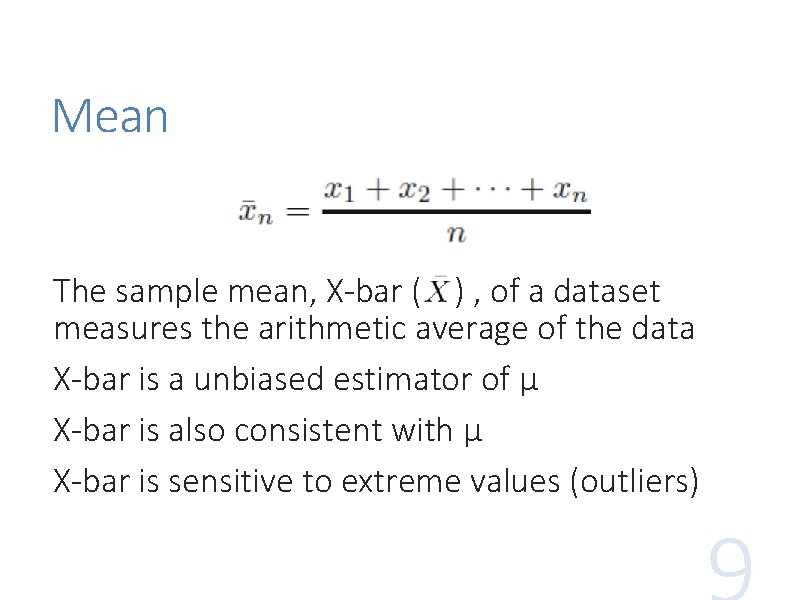
Mean The sample mean, X-bar ( ) , of a dataset measures the arithmetic average of the data X-bar is a unbiased estimator of μ X-bar is also consistent with μ X-bar is sensitive to extreme values (outliers)

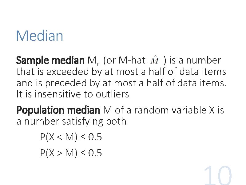
Median Sample median Mn (or M-hat ) is a number that is exceeded by at most a half of data items and is preceded by at most a half of data items. It is insensitive to outliers Population median M of a random variable X is a number satisfying both P(X < M) ≤ 0. 5 P(X > M) ≤ 0. 5

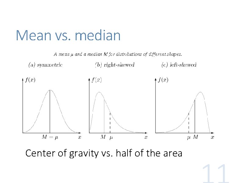
Mean vs. median Center of gravity vs. half of the area

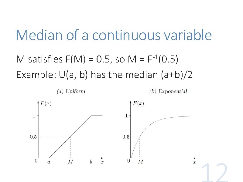
Median of a continuous variable M satisfies F(M) = 0. 5, so M = F-1(0. 5) Example: U(a, b) has the median (a+b)/2

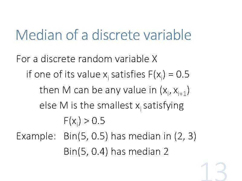
Median of a discrete variable For a discrete random variable X if one of its value xi satisfies F(xi) = 0. 5 then M can be any value in (xi, xi+1) else M is the smallest xi satisfying F(xi) > 0. 5 Example: Bin(5, 0. 5) has median in (2, 3) Bin(5, 0. 4) has median 2

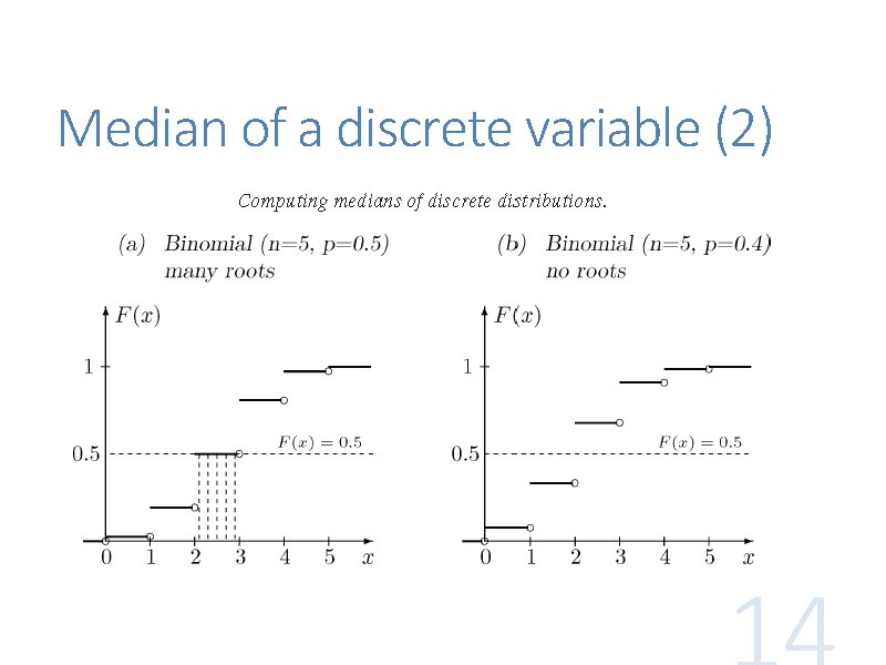
Median of a discrete variable (2)

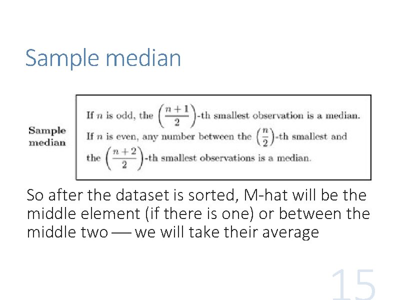
Sample median So after the dataset is sorted, M-hat will be the middle element (if there is one) or between the middle two we will take their average

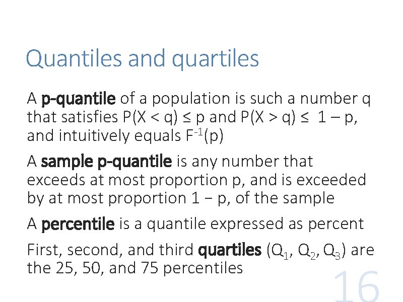
Quantiles and quartiles A p-quantile of a population is such a number q that satisfies P(X < q) ≤ p and P(X > q) ≤ 1 – p, and intuitively equals F-1(p) A sample p-quantile is any number that exceeds at most proportion p, and is exceeded by at most proportion 1 − p, of the sample A percentile is a quantile expressed as percent First, second, and third quartiles (Q 1, Q 2, Q 3) are the 25, 50, and 75 percentiles

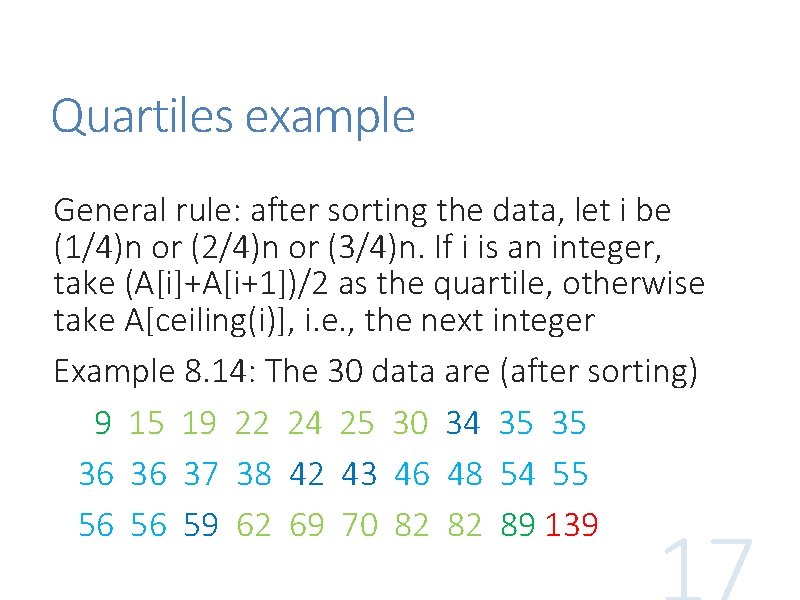
Quartiles example General rule: after sorting the data, let i be (1/4)n or (2/4)n or (3/4)n. If i is an integer, take (A[i]+A[i+1])/2 as the quartile, otherwise take A[ceiling(i)], i. e. , the next integer Example 8. 14: The 30 data are (after sorting) 9 15 19 22 24 25 30 34 35 35 36 36 37 38 42 43 46 48 54 55 56 56 59 62 69 70 82 82 89 139

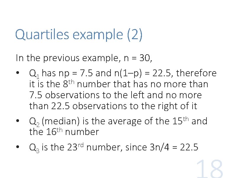
Quartiles example (2) In the previous example, n = 30, • Q 1 has np = 7. 5 and n(1–p) = 22. 5, therefore it is the 8 th number that has no more than 7. 5 observations to the left and no more than 22. 5 observations to the right of it • Q 2 (median) is the average of the 15 th and the 16 th number • Q 3 is the 23 rd number, since 3 n/4 = 22. 5

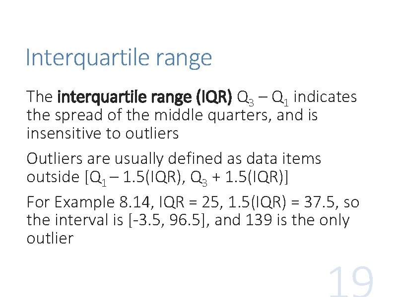
Interquartile range The interquartile range (IQR) Q 3 – Q 1 indicates the spread of the middle quarters, and is insensitive to outliers Outliers are usually defined as data items outside [Q 1 – 1. 5(IQR), Q 3 + 1. 5(IQR)] For Example 8. 14, IQR = 25, 1. 5(IQR) = 37. 5, so the interval is [-3. 5, 96. 5], and 139 is the only outlier

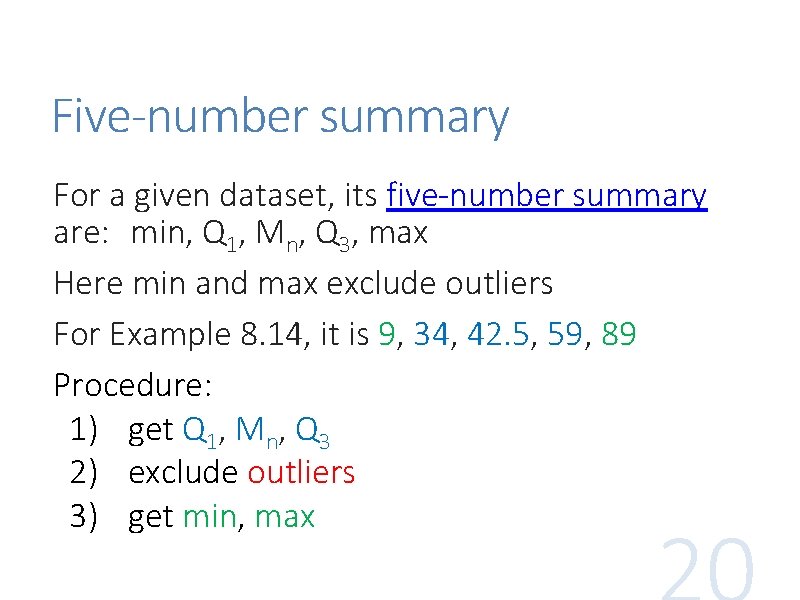
Five-number summary For a given dataset, its five-number summary are: min, Q 1, Mn, Q 3, max Here min and max exclude outliers For Example 8. 14, it is 9, 34, 42. 5, 59, 89 Procedure: 1) get Q 1, Mn, Q 3 2) exclude outliers 3) get min, max

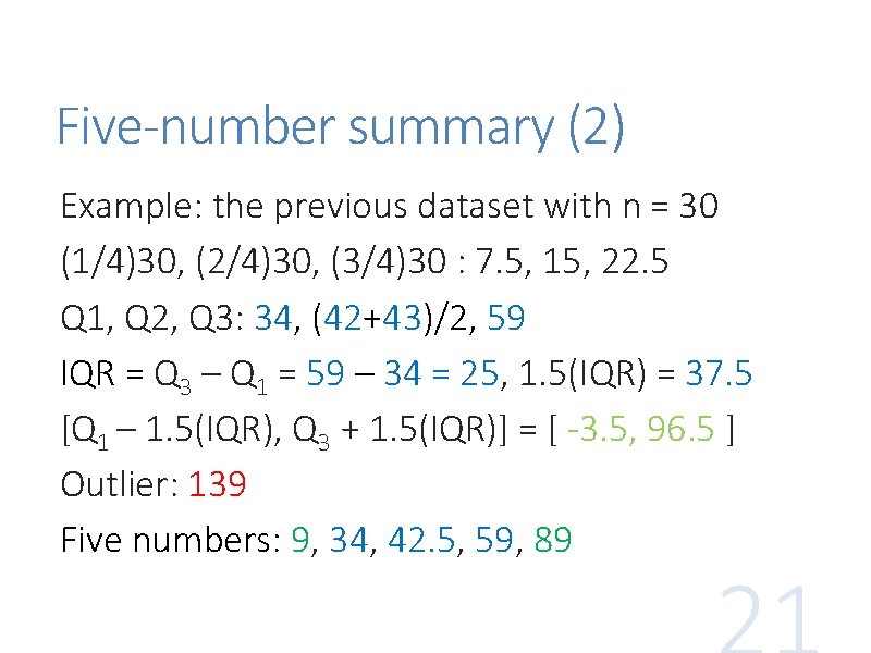
Five-number summary (2) Example: the previous dataset with n = 30 (1/4)30, (2/4)30, (3/4)30 : 7. 5, 15, 22. 5 Q 1, Q 2, Q 3: 34, (42+43)/2, 59 IQR = Q 3 – Q 1 = 59 – 34 = 25, 1. 5(IQR) = 37. 5 [Q 1 – 1. 5(IQR), Q 3 + 1. 5(IQR)] = [ -3. 5, 96. 5 ] Outlier: 139 Five numbers: 9, 34, 42. 5, 59, 89

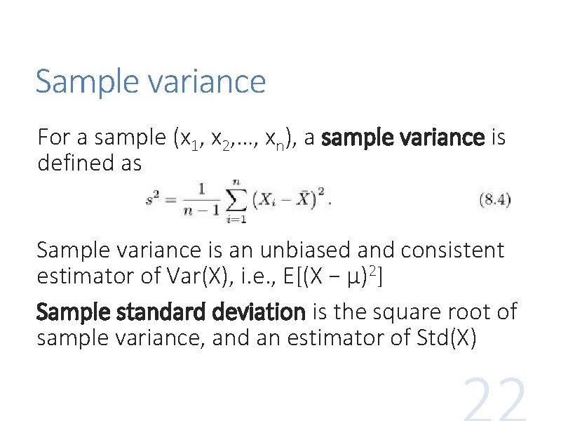
Sample variance For a sample (x 1, x 2, …, xn), a sample variance is defined as Sample variance is an unbiased and consistent estimator of Var(X), i. e. , E[(X − µ)2] Sample standard deviation is the square root of sample variance, and an estimator of Std(X)

Sample variance (2) Similar to Var(X) = E[X 2] − µ 2, it is easier to use Many calculators and statistics software provide procedures to calculate sample variance and/or sample standard deviation

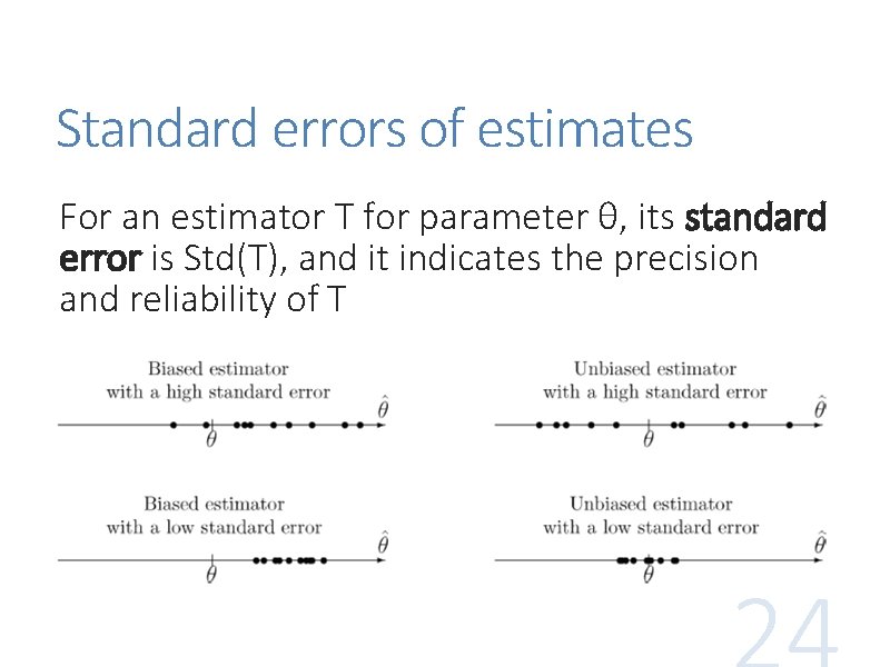
Standard errors of estimates For an estimator T for parameter θ, its standard error is Std(T), and it indicates the precision and reliability of T

Summary of descriptive statistics The simple descriptive (numerical) statistics introduced so far belong to two systems: 1. With mean for center and variance / standard deviation for spread 2. With median for center and quartiles / IQR / five-number summary for spread Either system can be applied to the sample (data), as well as to the population (model)

Graphical statistics A quick look at a graph of a dataset may clearly suggest • a probability model • statistical methods suitable for the data • presence or absence of outliers • existence of patterns • relation between two or several variables

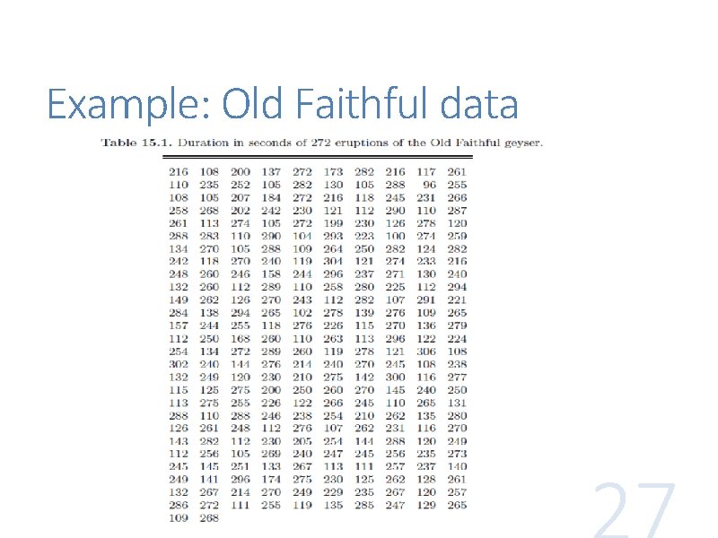
Example: Old Faithful data

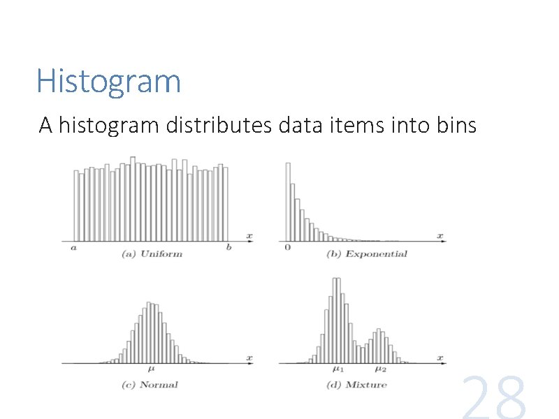
Histogram A histogram distributes data items into bins

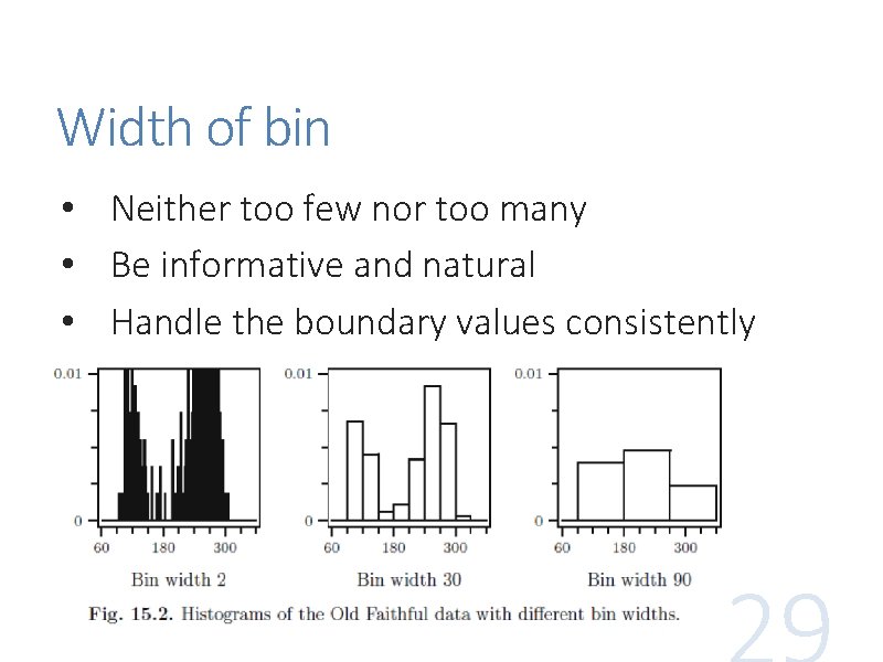
Width of bin • Neither too few nor too many • Be informative and natural • Handle the boundary values consistently

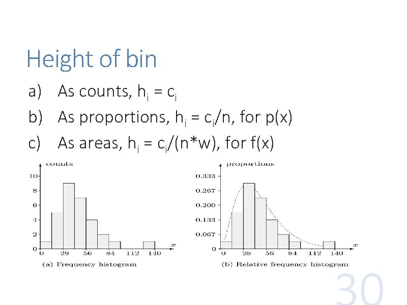
Height of bin a) As counts, hi = ci b) As proportions, hi = ci/n, for p(x) c) As areas, hi = ci/(n*w), for f(x)

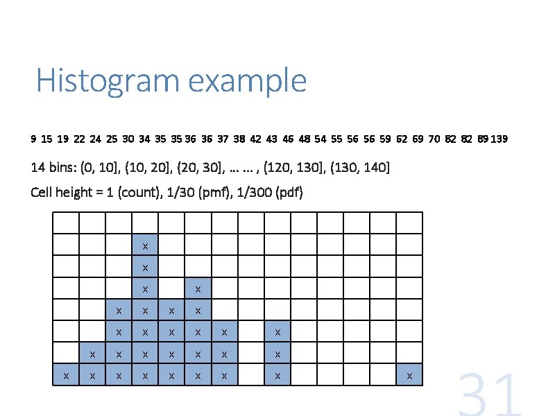
Histogram example 9 15 19 22 24 25 30 34 35 35 36 36 37 38 42 43 46 48 54 55 56 56 59 62 69 70 82 82 89 139 14 bins: (0, 10], (10, 20], (20, 30], …. . . , (120, 130], (130, 140] Cell height = 1 (count), 1/30 (pmf), 1/300 (pdf) x x x x x x x x

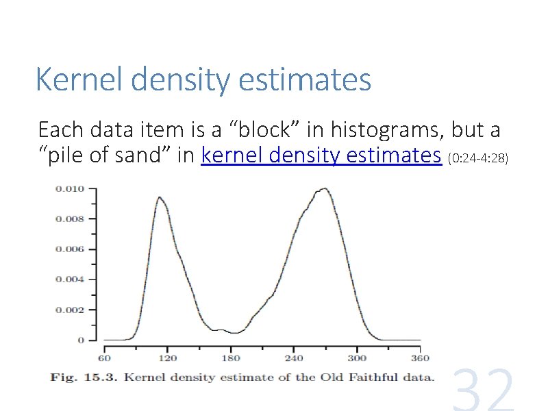
Kernel density estimates Each data item is a “block” in histograms, but a “pile of sand” in kernel density estimates (0: 24 -4: 28)

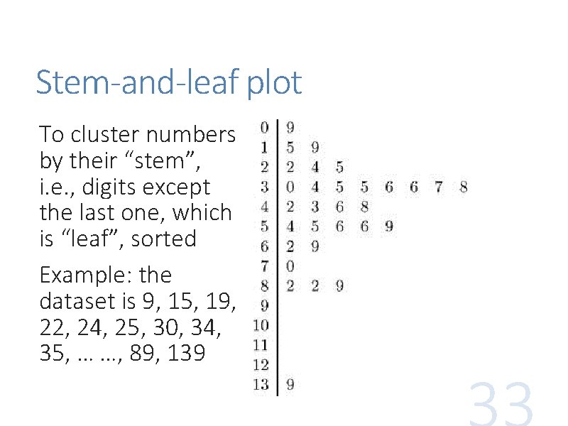
Stem-and-leaf plot To cluster numbers by their “stem”, i. e. , digits except the last one, which is “leaf”, sorted Example: the dataset is 9, 15, 19, 22, 24, 25, 30, 34, 35, … …, 89, 139

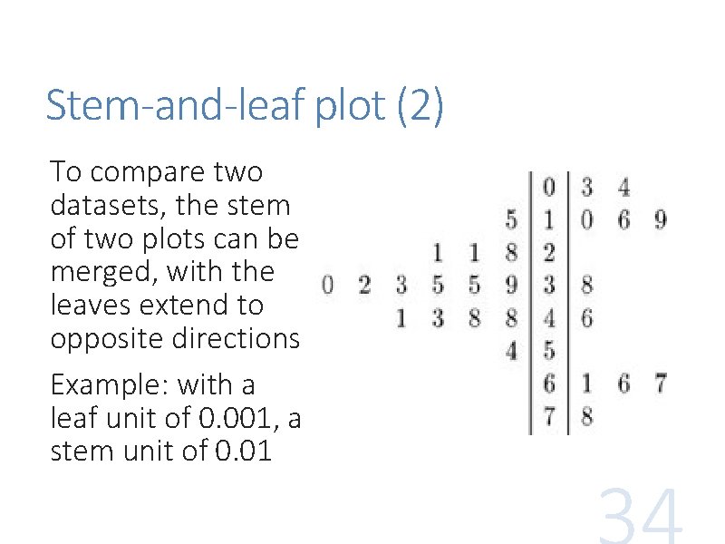
Stem-and-leaf plot (2) To compare two datasets, the stem of two plots can be merged, with the leaves extend to opposite directions Example: with a leaf unit of 0. 001, a stem unit of 0. 01

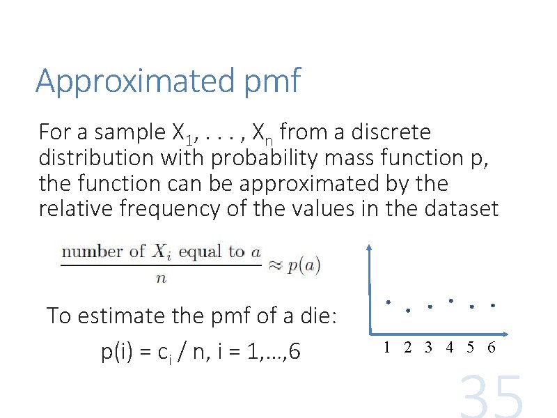
Approximated pmf For a sample X 1, . . . , Xn from a discrete distribution with probability mass function p, the function can be approximated by the relative frequency of the values in the dataset To estimate the pmf of a die: p(i) = ci / n, i = 1, …, 6 1 2 3 4 5 6

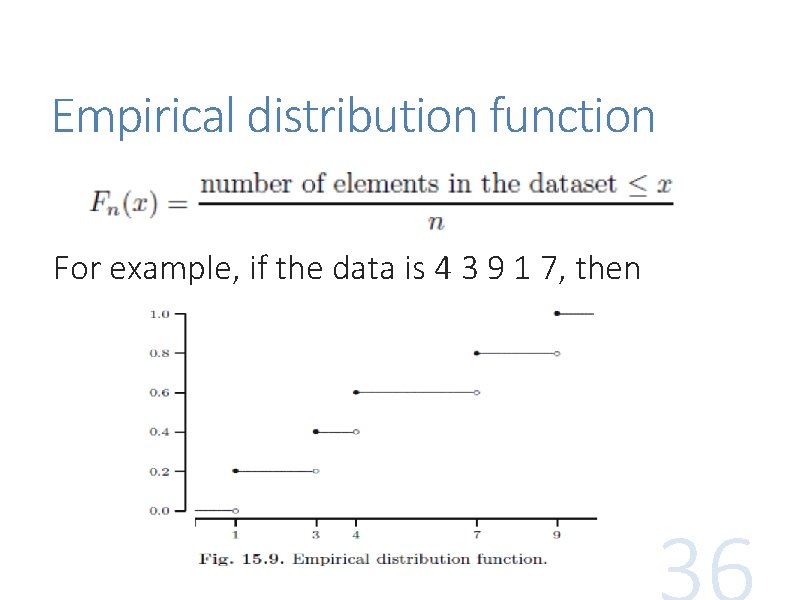
Empirical distribution function For example, if the data is 4 3 9 1 7, then

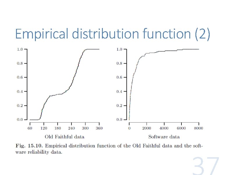
Empirical distribution function (2)

Boxplot (a. k. a. box-and-whisker plot) shows the five-number summary of a dataset: min, Q 1, Mn, Q 3, max In a boxplot, the box is from Q 1 to Q 3, with Mn as a bar in the middle. Optionally, mean is at ‘+’ The two whiskers from the box extend to the min and max, respectively Outliers are drawn separately as circles or dots

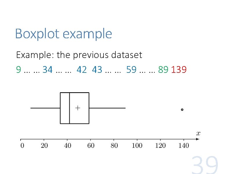
Boxplot example Example: the previous dataset 9 … … 34 … … 42 43 … … 59 … … 89 139

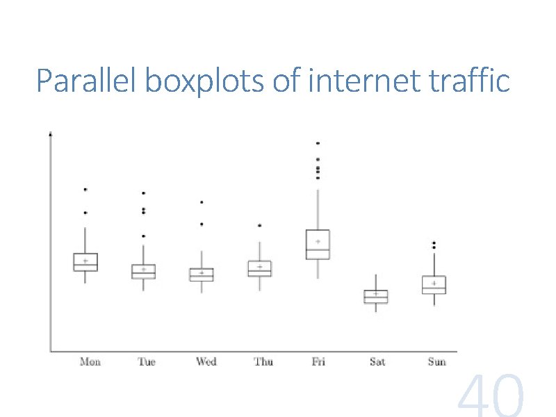
Parallel boxplots of internet traffic

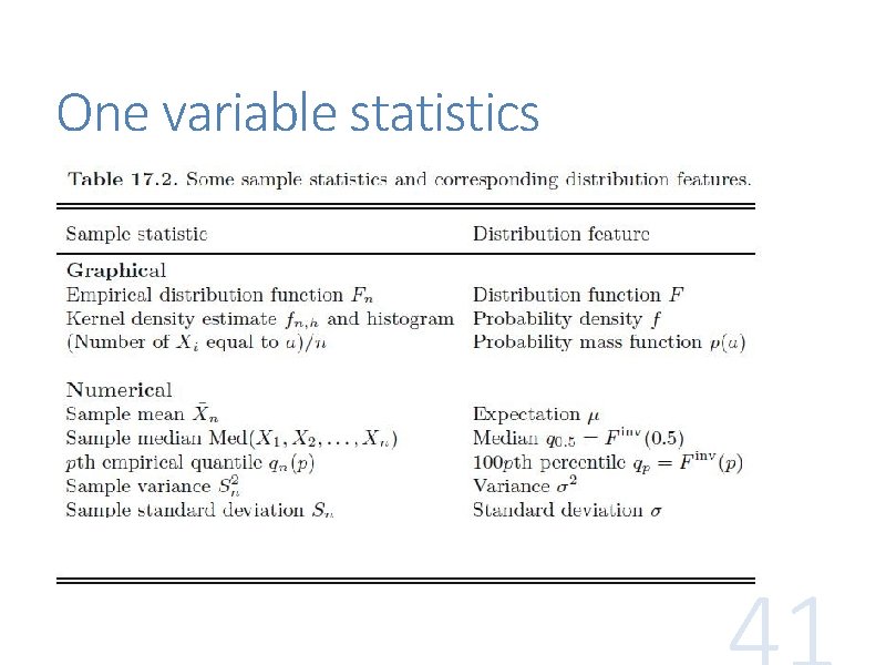
One variable statistics

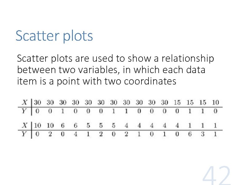
Scatter plots are used to show a relationship between two variables, in which each data item is a point with two coordinates

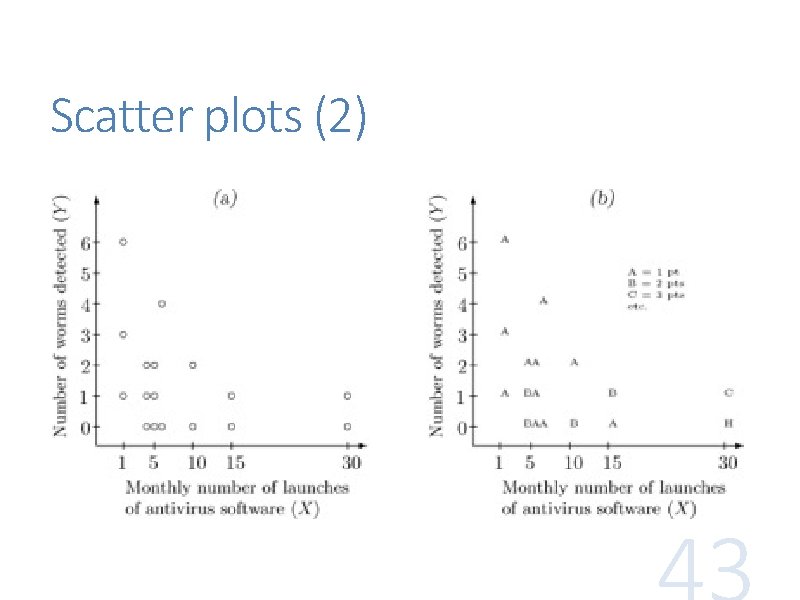
Scatter plots (2)

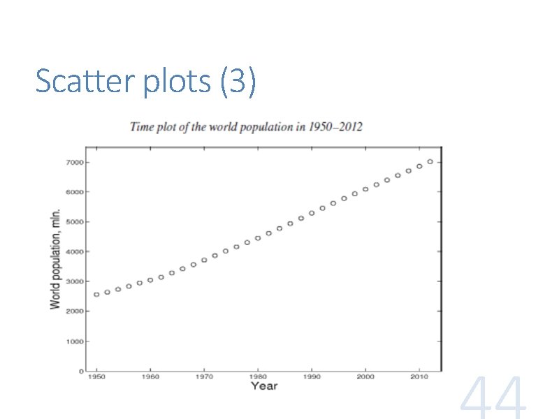
Scatter plots (3)