Probability and Random Variables Why Probability in Communications

Probability and Random Variables Ø Ø Ø Why Probability in Communications Probability Random Variables Probability Density Functions Cumulative Distribution Functions Huseyin Bilgekul EEE 461 Communication Systems II Department of Electrical and Electronic Engineering Eastern Mediterranean University EEE 461 1

Why probability in Communications? • Modeling effects of noise – quantization – Channel – Thermal • What happens when noise and signal are filtered, mixed, etc? • Making the “best” decision at the receiver EEE 461 2

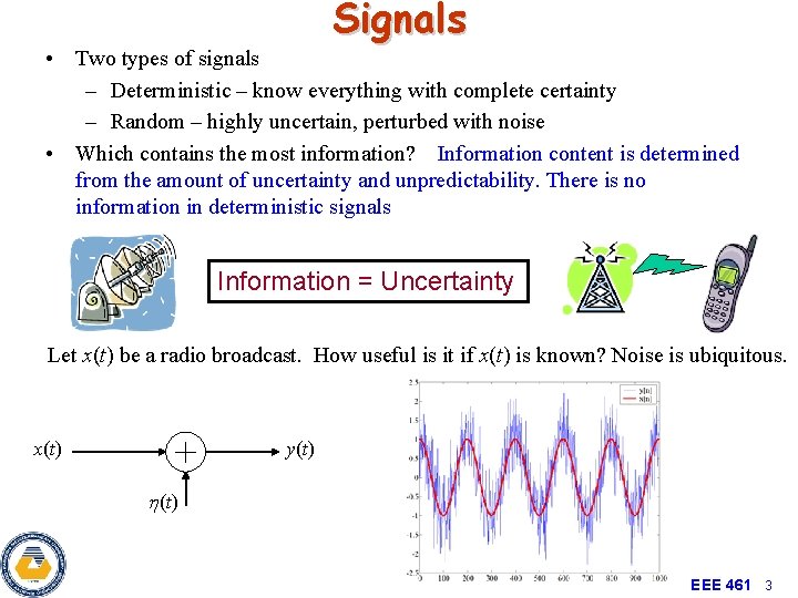
Signals • Two types of signals – Deterministic – know everything with complete certainty – Random – highly uncertain, perturbed with noise • Which contains the most information? Information content is determined from the amount of uncertainty and unpredictability. There is no information in deterministic signals Information = Uncertainty Let x(t) be a radio broadcast. How useful is it if x(t) is known? Noise is ubiquitous. x(t) y(t) h(t) EEE 461 3

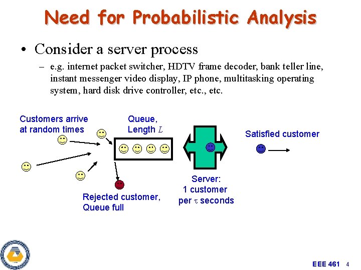
Need for Probabilistic Analysis • Consider a server process – e. g. internet packet switcher, HDTV frame decoder, bank teller line, instant messenger video display, IP phone, multitasking operating system, hard disk drive controller, etc. Customers arrive at random times Queue, Length L Rejected customer, Queue full Satisfied customer Server: 1 customer per seconds EEE 461 4

Probability Definitions • Random Experiment – outcome cannot be precisely predicted due to complexity • Outcomes – results of random experiment • Events – sets of outcomes that meet a criteria, roll of a die greater than 4 • Sample Space – set of all possible outcomes, E (sometimes called the Universal Set) EEE 461 5

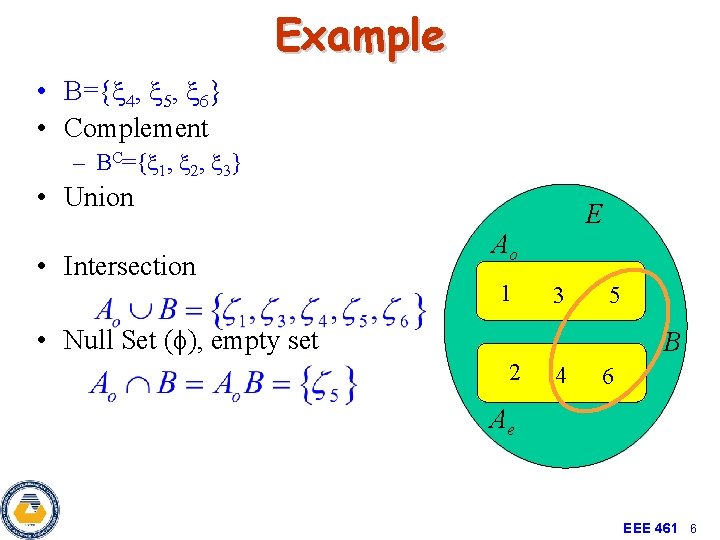
Example • B={x 4, x 5, x 6} • Complement – BC={x 1, x 2, x 3} • Union • Intersection E Ao 1 3 5 • Null Set (f), empty set B 2 4 6 Ae EEE 461 6

Relative Frequency • n. A – number of elements in a set, e. g. the number of times an event occurs in N trials • Probability is related to the relative frequency • For N small, fraction varies a lot; usually gets better as N increases EEE 461 7

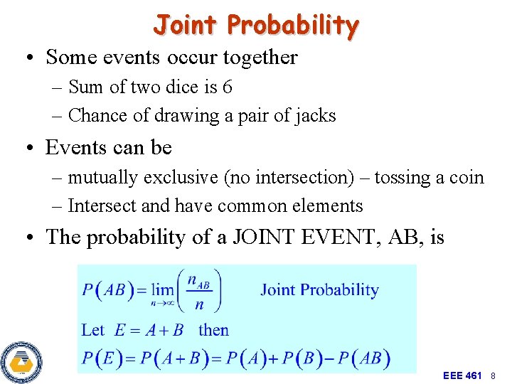
Joint Probability • Some events occur together – Sum of two dice is 6 – Chance of drawing a pair of jacks • Events can be – mutually exclusive (no intersection) – tossing a coin – Intersect and have common elements • The probability of a JOINT EVENT, AB, is EEE 461 8

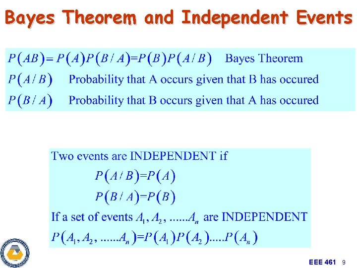
Bayes Theorem and Independent Events EEE 461 9

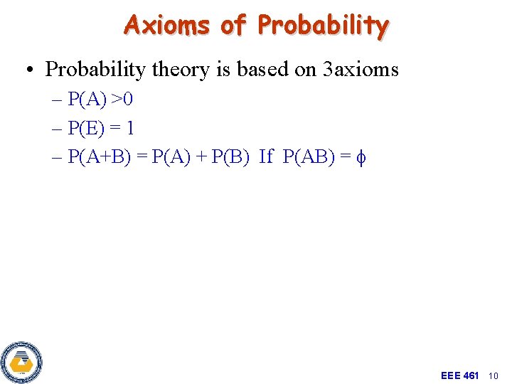
Axioms of Probability • Probability theory is based on 3 axioms – P(A) >0 – P(E) = 1 – P(A+B) = P(A) + P(B) If P(AB) = f EEE 461 10

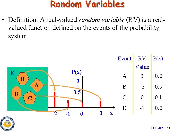
Random Variables • Definition: A real-valued random variable (RV) is a realvalued function defined on the events of the probability system Event E B D P(x) 1 A 0. 5 C -2 -1 0 3 x RV P(x) Value A 3 0. 2 B -2 0. 5 C 0 0. 1 D -1 0. 2 EEE 461 11

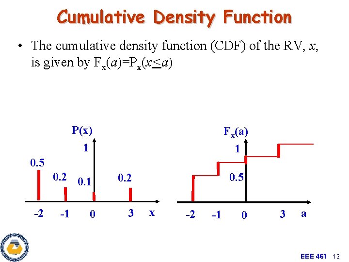
Cumulative Density Function • The cumulative density function (CDF) of the RV, x, is given by Fx(a)=Px(x<a) P(x) Fx(a) 1 1 0. 5 0. 2 0. 1 -2 -1 0 0. 5 0. 2 3 x -2 -1 0 3 a EEE 461 12

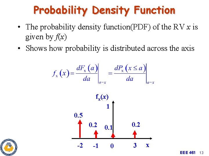
Probability Density Function • The probability density function(PDF) of the RV x is given by f(x) • Shows how probability is distributed across the axis fx(x) 1 0. 5 0. 2 0. 1 -2 -1 0 0. 2 3 x EEE 461 13

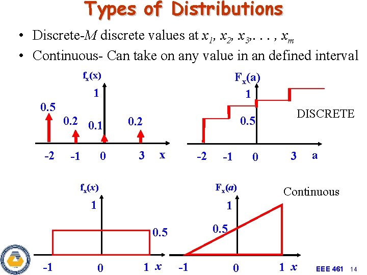
Types of Distributions • Discrete-M discrete values at x 1, x 2, x 3, . . . , xm • Continuous- Can take on any value in an defined interval fx(x) Fx(a) 1 1 0. 5 -2 0. 1 -1 0 0. 5 0. 2 3 x -2 fx(x) Fx(a) 1 0 3 a Continuous 1 0. 5 -1 -1 DISCRETE 0 1 x -1 0 1 x EEE 461 14

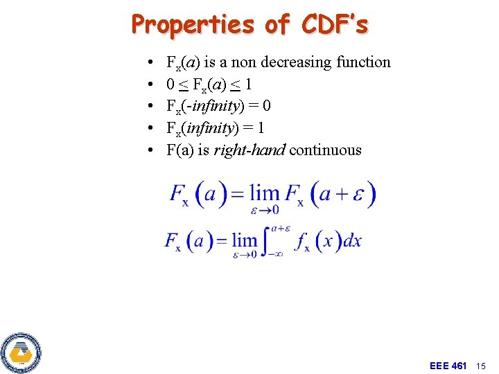
Properties of CDF’s • • • Fx(a) is a non decreasing function 0 < Fx(a) < 1 Fx(-infinity) = 0 Fx(infinity) = 1 F(a) is right-hand continuous EEE 461 15

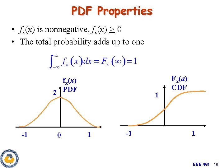
PDF Properties • fx(x) is nonnegative, fx(x) > 0 • The total probability adds up to one fx(x) 2 PDF -1 0 1 1 -1 Fx(a) CDF 1 EEE 461 16

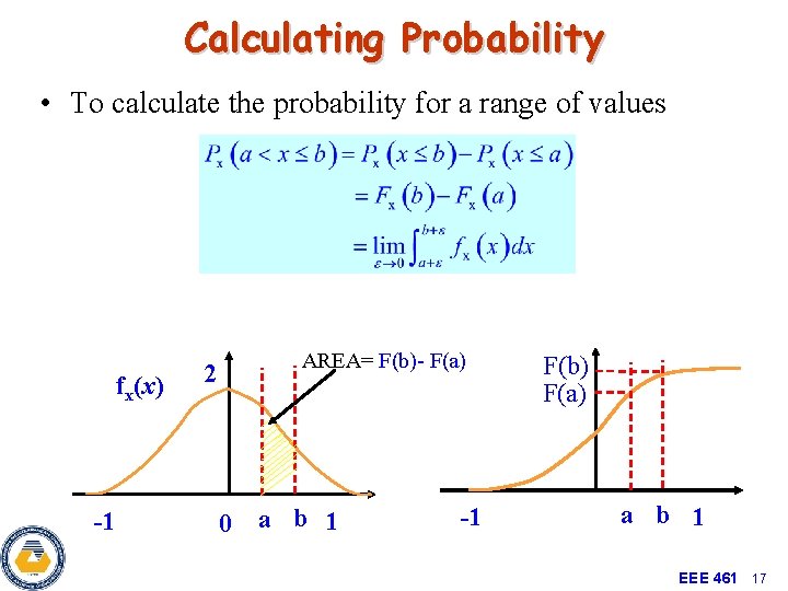
Calculating Probability • To calculate the probability for a range of values fx(x) -1 AREA= F(b)- F(a) 2 0 a b 1 -1 F(b) F(a) a b 1 EEE 461 17

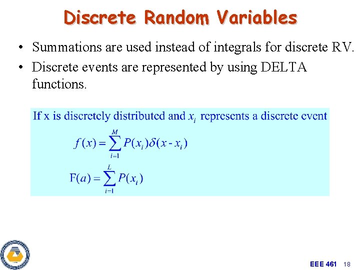
Discrete Random Variables • Summations are used instead of integrals for discrete RV. • Discrete events are represented by using DELTA functions. EEE 461 18

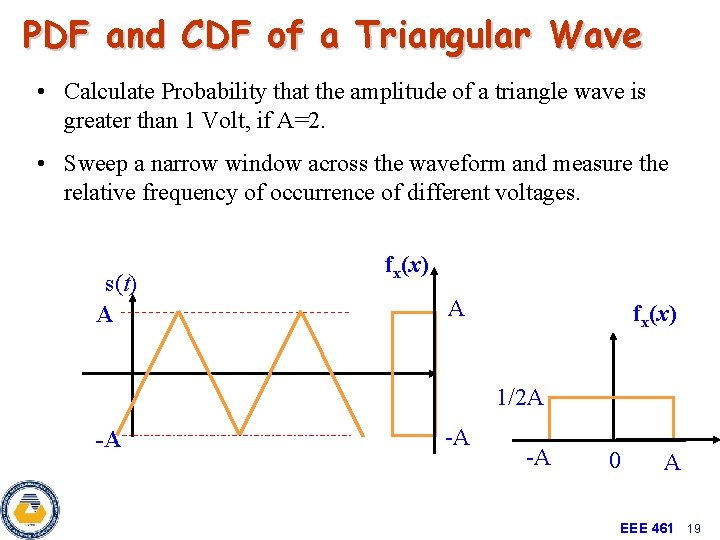
PDF and CDF of a Triangular Wave • Calculate Probability that the amplitude of a triangle wave is greater than 1 Volt, if A=2. • Sweep a narrow window across the waveform and measure the relative frequency of occurrence of different voltages. s(t) A fx(x) 1/2 A -A -A -A 0 A EEE 461 19

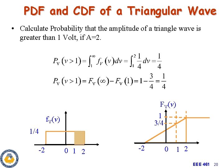
PDF and CDF of a Triangular Wave • Calculate Probability that the amplitude of a triangle wave is greater than 1 Volt, if A=2. FV(v) 1 3/4 f. V(v) 1/4 -2 0 1 2 EEE 461 20

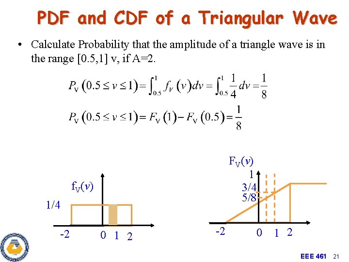
PDF and CDF of a Triangular Wave • Calculate Probability that the amplitude of a triangle wave is in the range [0. 5, 1] v, if A=2. FV(v) 1 3/4 5/8 f. V(v) 1/4 -2 0 1 2 EEE 461 21

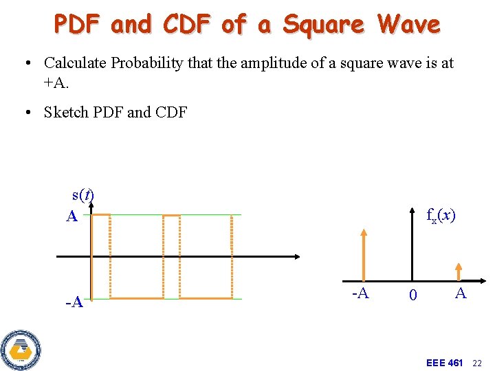
PDF and CDF of a Square Wave • Calculate Probability that the amplitude of a square wave is at +A. • Sketch PDF and CDF s(t) A -A fx(x) -A 0 A EEE 461 22

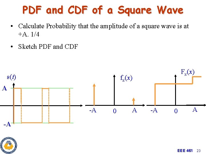
PDF and CDF of a Square Wave • Calculate Probability that the amplitude of a square wave is at +A. 1/4 • Sketch PDF and CDF s(t) Fx(x) fx(x) A -A 0 A -A EEE 461 23

Ensemble Averages • The expected value (or ensemble average) of y=h(x) is: EEE 461 24

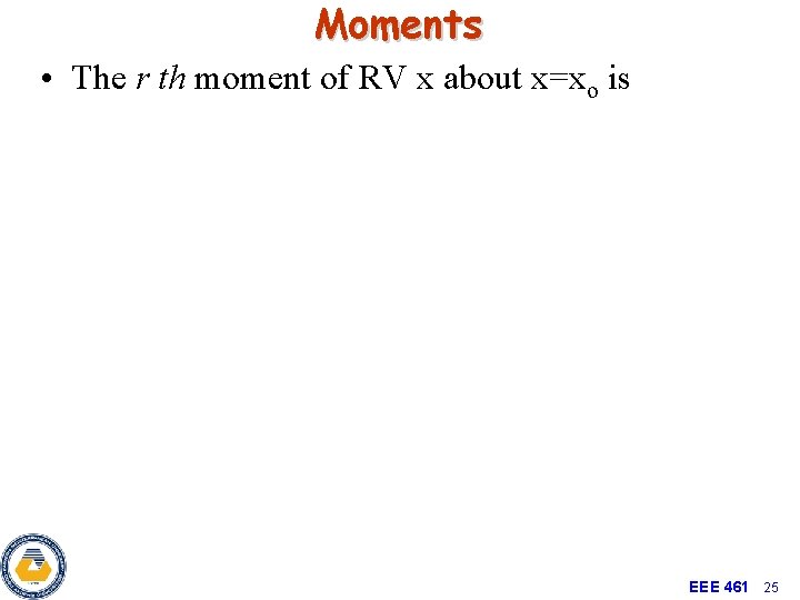
Moments • The r th moment of RV x about x=xo is EEE 461 25