PROBABILITY AND PROBABILITY DISTRIBUTIONS 1 What is probability

PROBABILITY AND PROBABILITY DISTRIBUTIONS 1

What is probability? Probability: • Provides a measure of the uncertainty (or certainty) associated with the occurrence of events or outcomes. • The chance that an uncertain event will occur • Likelihood of an event • Assumes a random process: i. e. . the outcome is not predetermined - there is an element of chance • It is useful in exploring and quantifying relationships • Winning the “Enkutatash” Lottery • Heads every time in 24 tosses of a coin 2

Example 5. 1 1. Consider an experiment of tossing a coin a. what is the probability of observing head b. what is the probability of observing tail Solution First list all possible values, sample space, of the experiment S={H, T} Then P(H)=1/2=0. 5 Then P(T)=1/2=0. 5 3

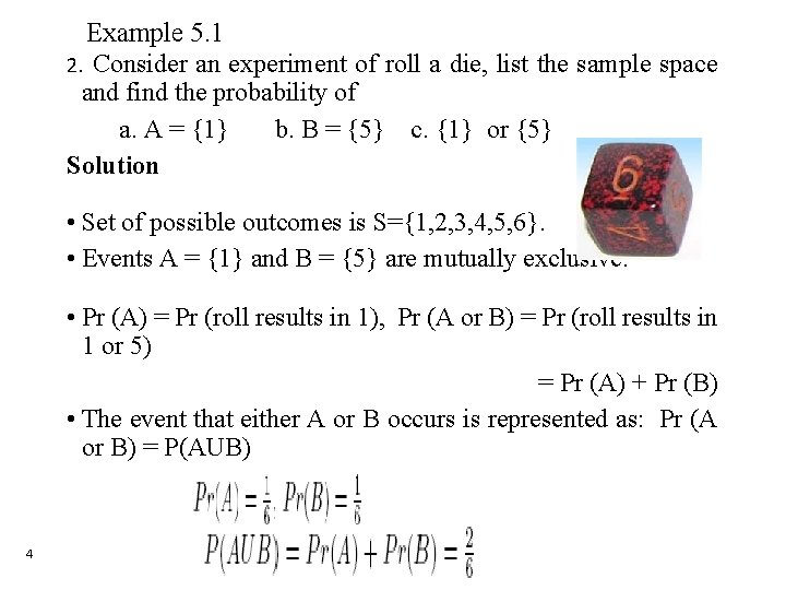
Example 5. 1 2. Consider an experiment of roll a die, list the sample space and find the probability of a. A = {1} b. B = {5} c. {1} or {5} Solution • Set of possible outcomes is S={1, 2, 3, 4, 5, 6}. • Events A = {1} and B = {5} are mutually exclusive. • Pr (A) = Pr (roll results in 1), Pr (A or B) = Pr (roll results in 1 or 5) = Pr (A) + Pr (B) • The event that either A or B occurs is represented as: Pr (A or B) = P(AUB) 4

Why We Study Probability? • To investigate how much information contained in the sample can be used to infer the characteristics of the population. • For generalization 5

Basic terms • Experiment : anything that results in a count or a measurement. In other words a situation involving chance or probability that leads to results called outcomes. • Sample space : The set of all possible outcomes of an experiment , Example: (H, T) of a coin. • Event : Something that may happen or not when the experiment is performed. Any subset of the sample space H or T.

Con’t… • Outcome: a specific result of a single trial of an experiment. • A set : a collection of objects. The objects in a set are called the elements of the set. • Mutually exclusive events: Two events A and B are mutually exclusive if they have no elements in common. If A and B are outcomes of an experiment they cannot both happen at the same time. • Independence Event: The probability of one factor is not affected by the state of another factor.

Types of probability 1. The Classical Probability • If there are n equally likely possibilities, of which one must occur and m are regarded as favorable, or as a “success” then the probability of a “success” is m/n. • In other words if the number of outcomes belonging to an event E is NE , and the total number of outcomes is N, then the probability of 8 event E is defined as : P(E)=NE /N

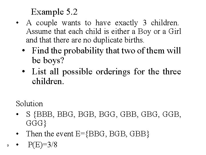
Example 5. 2 • A couple wants to have exactly 3 children. Assume that each child is either a Boy or a Girl and that there are no duplicate births. • Find the probability that two of them will be boys? • List all possible orderings for the three children. 9 Solution • S {BBB, BBG, BGB, BGG, GBB, GBG, GGB, GGG} • Then the event E={BBG, BGB, GBB} • P(E)=3/8

Types of probability Cont… 2. Relative Frequency Probabilities • This approach to probability is well-suited to a wide range of scientific disciplines. • It is based on the idea that the underlying probability of an event can be measured by repeated trials. • Frequentist definition of probability says the probability that something occurs is the proportion of times it occurs when exactly the same experiment is repeated a very large (preferably infinite!) number of times in independent trials. 1 0

Types of probability Cont… 3. Subjective probability • In this view, probability is treated as a quantifiable level of belief ranging from 0 (complete disbelief) to 1 (complete belief) • For instance, an experienced physician may say “ this patient has a 50% chance of recovery. ” • An appreciation of the various types of probability are not mutually exclusive. And fortunately, all obey the same, mathematical laws, and their methods of calculation are similar. 1 1 • All probabilities are a type of relative frequency i. e the number of times something can occur divided by the total number of possibilities or occurrences.

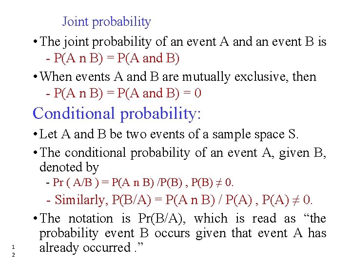
Joint probability • The joint probability of an event A and an event B is - P(A n B) = P(A and B) • When events A and B are mutually exclusive, then - P(A n B) = P(A and B) = 0 Conditional probability: • Let A and B be two events of a sample space S. • The conditional probability of an event A, given B, denoted by - Pr ( A/B ) = P(A n B) /P(B) , P(B) ≠ 0. 1 2 - Similarly, P(B/A) = P(A n B) / P(A) , P(A) ≠ 0. • The notation is Pr(B/A), which is read as “the probability event B occurs given that event A has already occurred. ”

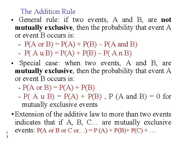
1 3 The Addition Rule • General rule: if two events, A and B, are not mutually exclusive, then the probability that event A or event B occurs is: - P(A or B) = P(A) + P(B) – P(A and B) - P( A u B) = P(A) + P(B) – P( A n B) • Special case: when two events, A and B, are mutually exclusive, then the probability that event A or event B occurs is: - P(A or B) = P(A) + P(B) - P( A u B) = P(A) + P(B) , P (A and B) = 0 for mutually exclusive events • Extension of the additive law to more than two events indicates that if A, B, C… are mutually exclusive events: P(A or B or C or…) = P (A) + P(B)+ P(C) + …

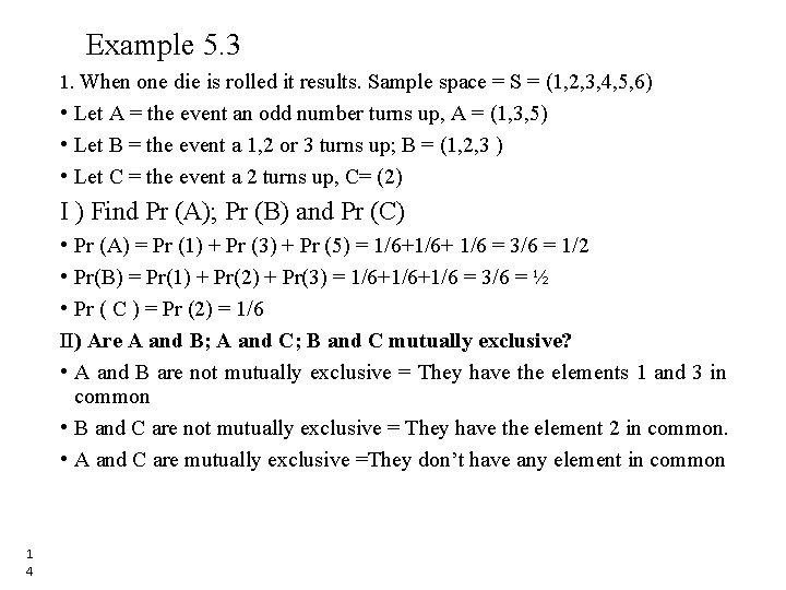
Example 5. 3 1. When one die is rolled it results. Sample space = S = (1, 2, 3, 4, 5, 6) • Let A = the event an odd number turns up, A = (1, 3, 5) • Let B = the event a 1, 2 or 3 turns up; B = (1, 2, 3 ) • Let C = the event a 2 turns up, C= (2) I ) Find Pr (A); Pr (B) and Pr (C) • Pr (A) = Pr (1) + Pr (3) + Pr (5) = 1/6+ 1/6 = 3/6 = 1/2 • Pr(B) = Pr(1) + Pr(2) + Pr(3) = 1/6+1/6 = 3/6 = ½ • Pr ( C ) = Pr (2) = 1/6 II) Are A and B; A and C; B and C mutually exclusive? • A and B are not mutually exclusive = They have the elements 1 and 3 in common • B and C are not mutually exclusive = They have the element 2 in common. • A and C are mutually exclusive =They don’t have any element in common 1 4

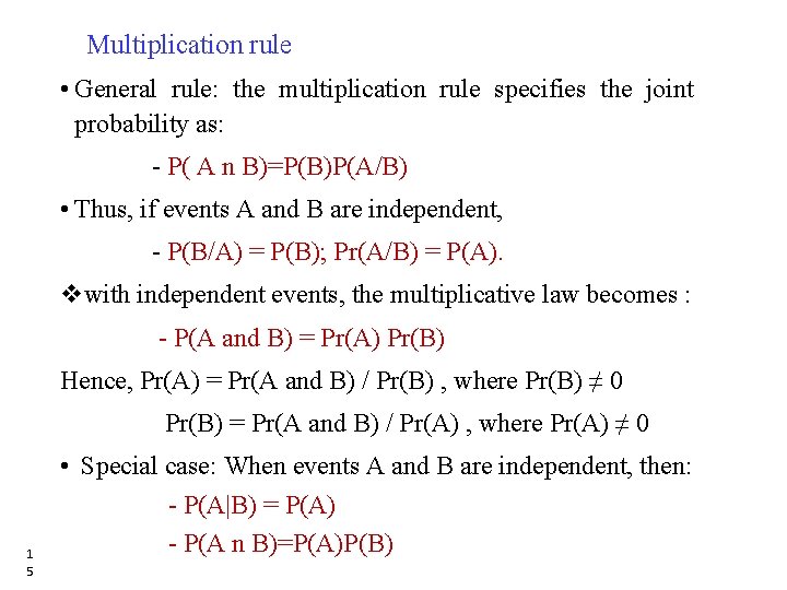
Multiplication rule • General rule: the multiplication rule specifies the joint probability as: - P( A n B)=P(B)P(A/B) • Thus, if events A and B are independent, - P(B/A) = P(B); Pr(A/B) = P(A). vwith independent events, the multiplicative law becomes : - P(A and B) = Pr(A) Pr(B) Hence, Pr(A) = Pr(A and B) / Pr(B) , where Pr(B) ≠ 0 Pr(B) = Pr(A and B) / Pr(A) , where Pr(A) ≠ 0 1 5 • Special case: When events A and B are independent, then: - P(A|B) = P(A) - P(A n B)=P(A)P(B)

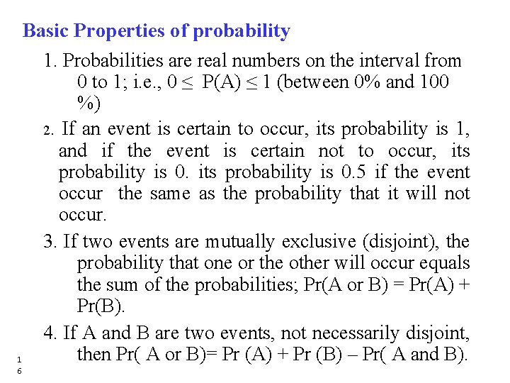
Basic Properties of probability 1. Probabilities are real numbers on the interval from 0 to 1; i. e. , 0 ≤ P(A) ≤ 1 (between 0% and 100 %) 2. If an event is certain to occur, its probability is 1, and if the event is certain not to occur, its probability is 0. 5 if the event occur the same as the probability that it will not occur. 3. If two events are mutually exclusive (disjoint), the probability that one or the other will occur equals the sum of the probabilities; Pr(A or B) = Pr(A) + Pr(B). 4. If A and B are two events, not necessarily disjoint, then Pr( A or B)= Pr (A) + Pr (B) – Pr( A and B). 1 6

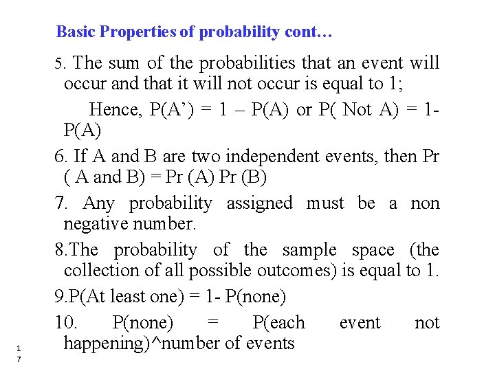
Basic Properties of probability cont… 5. The sum of the probabilities that an event will 1 7 occur and that it will not occur is equal to 1; Hence, P(A’) = 1 – P(A) or P( Not A) = 1 - P(A) 6. If A and B are two independent events, then Pr ( A and B) = Pr (A) Pr (B) 7. Any probability assigned must be a non negative number. 8. The probability of the sample space (the collection of all possible outcomes) is equal to 1. 9. P(At least one) = 1 - P(none) 10. P(none) = P(each event not happening)^number of events

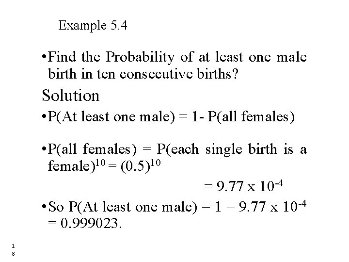
Example 5. 4 • Find the Probability of at least one male birth in ten consecutive births? Solution • P(At least one male) = 1 - P(all females) • P(all females) = P(each single birth is a female)10 = (0. 5)10 = 9. 77 x 10 -4 • So P(At least one male) = 1 – 9. 77 x 10 -4 = 0. 999023. 1 8

Probability Distribution 1 9

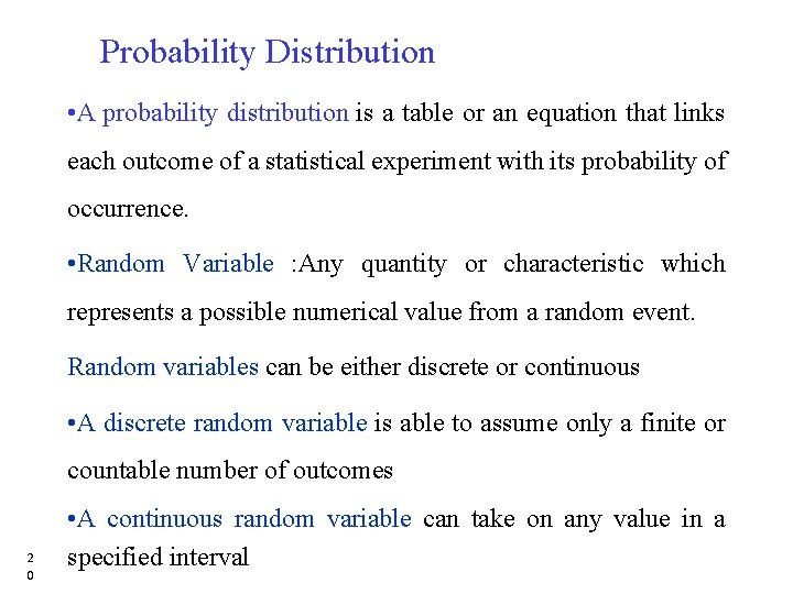
Probability Distribution • A probability distribution is a table or an equation that links each outcome of a statistical experiment with its probability of occurrence. • Random Variable : Any quantity or characteristic which represents a possible numerical value from a random event. Random variables can be either discrete or continuous • A discrete random variable is able to assume only a finite or countable number of outcomes 2 0 • A continuous random variable can take on any value in a specified interval

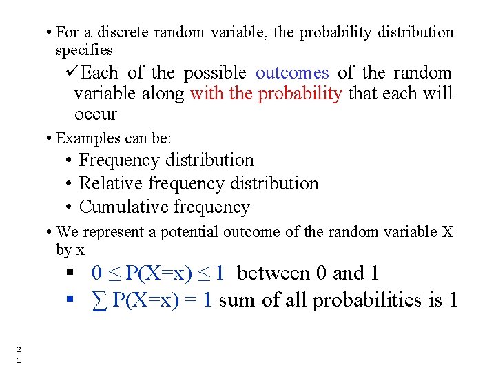
• For a discrete random variable, the probability distribution specifies üEach of the possible outcomes of the random variable along with the probability that each will occur • Examples can be: • Frequency distribution • Relative frequency distribution • Cumulative frequency • We represent a potential outcome of the random variable X by x § 0 ≤ P(X=x) ≤ 1 between 0 and 1 § ∑ P(X=x) = 1 sum of all probabilities is 1 2 1

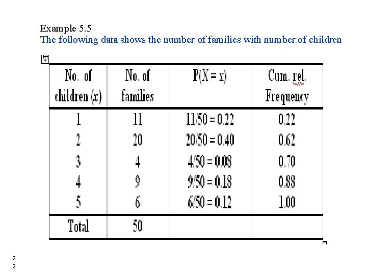
Example 5. 5 The following data shows the number of families with number of children 2 2

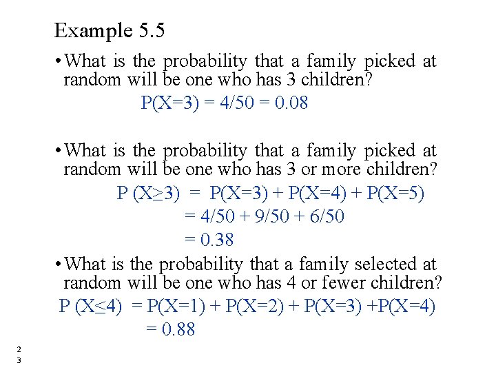
Example 5. 5 • What is the probability that a family picked at random will be one who has 3 children? P(X=3) = 4/50 = 0. 08 • What is the probability that a family picked at random will be one who has 3 or more children? P (X≥ 3) = P(X=3) + P(X=4) + P(X=5) = 4/50 + 9/50 + 6/50 = 0. 38 • What is the probability that a family selected at random will be one who has 4 or fewer children? P (X≤ 4) = P(X=1) + P(X=2) + P(X=3) +P(X=4) = 0. 88 2 3

Probability Distribution cont… Types of probability distributions of discrete variables: 1. Binomial distribution 2. Poisson distribution 2 4

1. Binomial Distribution • It is one of the most widely encountered discrete probability distributions. • When a single trial of an experiment can result in only one of two mutually exclusive outcomes (success or failure; dead or alive; sick or well, etc) • Helps to know what proportion of individuals in a population possesses a particular character; 2 5 E. g. the proportion of persons of a locality who are sick at a particular point in time.

A binomial probability distribution occurs when the following assumptions are met. 1. 2. 3. 4. 2 6 The procedure has a fixed number of trials. The trials must be independent. Each trial results in one of two possible, mutually exclusive, outcomes. Success and failure. The probability of a success, denoted by p, remains constant from trial to trial. The probability of a failure, 1 -p, = q.

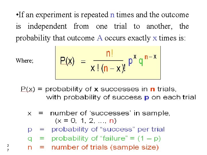
• If an experiment is repeated n times and the outcome is independent from one trial to another, the probability that outcome A occurs exactly x times is: Where; 2 7

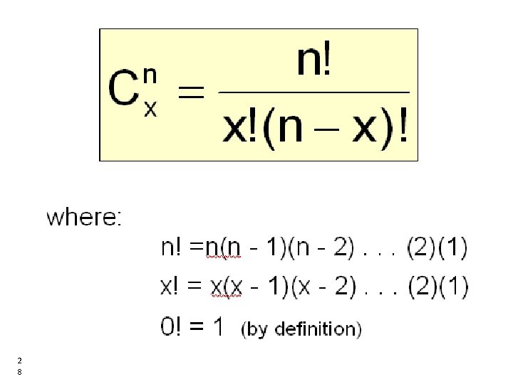
2 8

Example 5. 6 • Suppose we know that 40% of a certain population are cigarette smokers. • If we take a random sample of 10 people from this population, • What is the probability that we will have exactly 4 smokers in our sample? 2 9

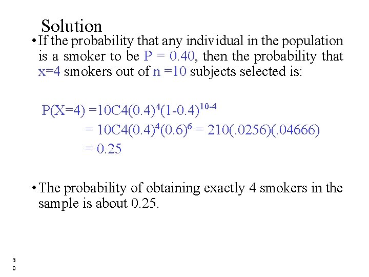
Solution • If the probability that any individual in the population is a smoker to be P = 0. 40, then the probability that x=4 smokers out of n =10 subjects selected is: P(X=4) =10 C 4(0. 4)4(1 -0. 4)10 -4 = 10 C 4(0. 4)4(0. 6)6 = 210(. 0256)(. 04666) = 0. 25 • The probability of obtaining exactly 4 smokers in the sample is about 0. 25. 3 0

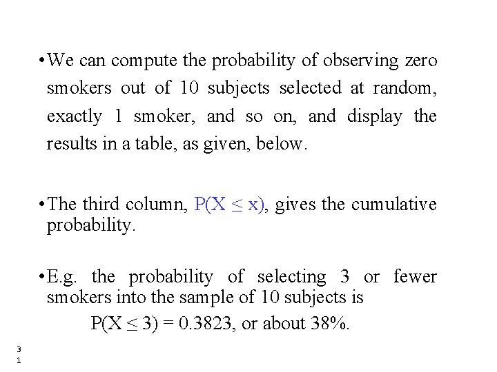
• We can compute the probability of observing zero smokers out of 10 subjects selected at random, exactly 1 smoker, and so on, and display the results in a table, as given, below. • The third column, P(X ≤ x), gives the cumulative probability. • E. g. the probability of selecting 3 or fewer smokers into the sample of 10 subjects is P(X ≤ 3) = 0. 3823, or about 38%. 3 1

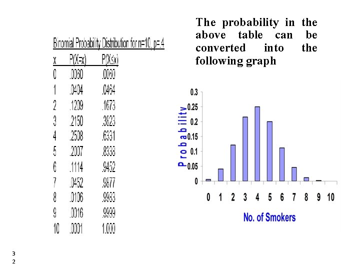
The probability in the above table can be converted into the following graph 3 2

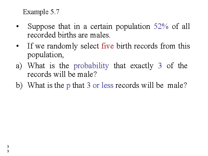
Example 5. 7 • Suppose that in a certain population 52% of all recorded births are males. • If we randomly select five birth records from this population, a) What is the probability that exactly 3 of the records will be male? b) What is the p that 3 or less records will be male? 3 3

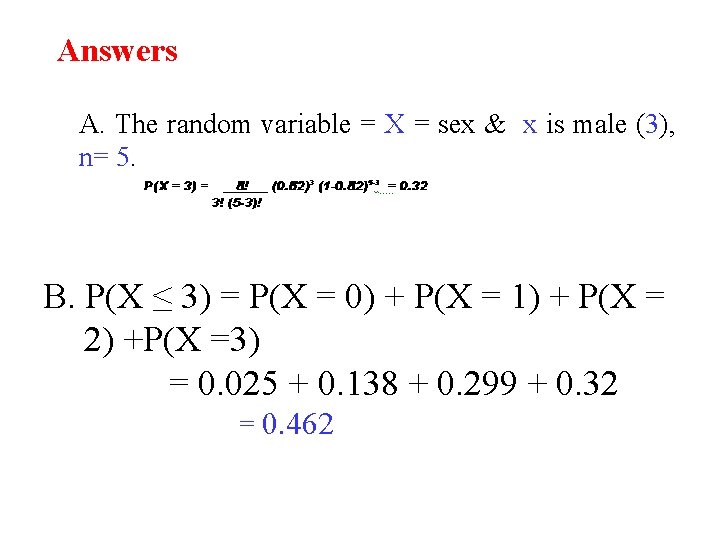
Answers A. The random variable = X = sex & x is male (3), n= 5. B. P(X ≤ 3) = P(X = 0) + P(X = 1) + P(X = 2) +P(X =3) = 0. 025 + 0. 138 + 0. 299 + 0. 32 = 0. 462

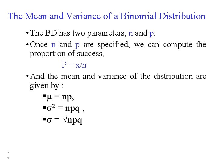
The Mean and Variance of a Binomial Distribution • The BD has two parameters, n and p. • Once n and p are specified, we can compute the proportion of success, P = x/n • And the mean and variance of the distribution are given by : §μ = np, §σ2 = npq , §σ = √npq 3 5

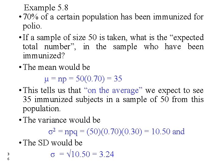
3 6 Example 5. 8 • 70% of a certain population has been immunized for polio. • If a sample of size 50 is taken, what is the “expected total number”, in the sample who have been immunized? • The mean would be µ = np = 50(0. 70) = 35 • This tells us that “on the average” we expect to see 35 immunized subjects in a sample of 50 from this population. • The variance would be σ2 = npq = (50)(0. 70)(0. 30) = 10. 50 and • The SD would be σ = √ 10. 50 = 3. 24

2. Poisson Distribution • The Poisson Distribution is a discrete distribution which takes on the values X = 0, 1, 2, 3, and so on. • It is often used as a model for the number of events in a specific time period. • It is determined by one parameter, lambda. 3 7

• The Poisson random variable satisfies the following conditions: • The number of successes in two disjoint time intervals is independent. • The probability of a success during a small time interval is proportional to the entire length of the time interval. • Eg. birth defects, genetic mutations, rare diseases (like Leukemia), car accidents, traffic flow and ideal gap distance, and so on

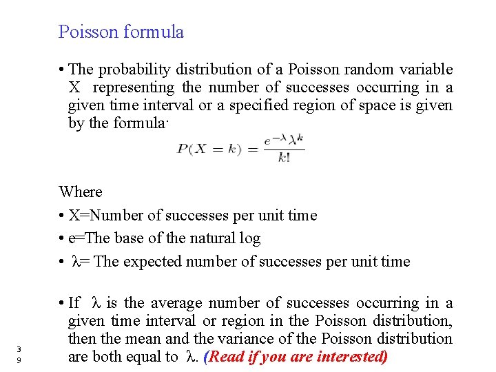
Poisson formula • The probability distribution of a Poisson random variable X representing the number of successes occurring in a given time interval or a specified region of space is given by the formula: Where • X=Number of successes per unit time • e=The base of the natural log • λ= The expected number of successes per unit time 3 9 • If λ is the average number of successes occurring in a given time interval or region in the Poisson distribution, then the mean and the variance of the Poisson distribution are both equal to λ. (Read if you are interested)

Probability Distribution for continuous Variables • If a random variable is a continuous variable, its probability distribution is called a continuous probability distribution. • Under different circumstances, the outcome of a random variable may not be limited to categories or counts. • Because a continuous random variable X can take on an uncountable infinite number of values, the probability associated with any particular one value is almost equal to zero. 4 0 • As a result, a continuous probability distribution cannot be expressed in tabular form.

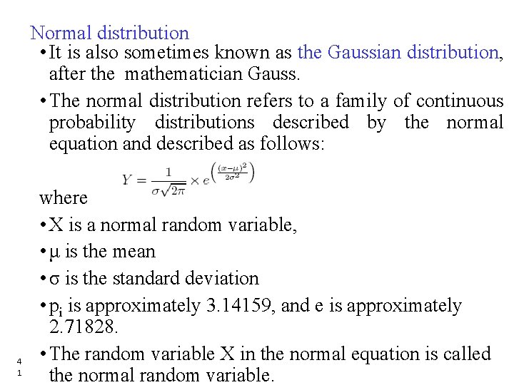
4 1 Normal distribution • It is also sometimes known as the Gaussian distribution, after the mathematician Gauss. • The normal distribution refers to a family of continuous probability distributions described by the normal equation and described as follows: where • X is a normal random variable, • μ is the mean • σ is the standard deviation • pi is approximately 3. 14159, and e is approximately 2. 71828. • The random variable X in the normal equation is called the normal random variable.

Characteristics of Normal Distribution 1. It links frequency distribution to probability distribution 2. It has a Bell Shape Curve , Unimodal and is Symmetric. 3. It is Symmetric around the mean: Two halves of the curve are the same (mirror images) , Hence Mean = Median 4. The total area under the curve is 1 (or 100%) 5. It is a probability distribution of a continuous variable. 6. It extends from minus infinity( -∞) to plus infinity (+∞). 7. It is determined by two quantities: Mean ( μ ) and SD ( σ ). 4 2

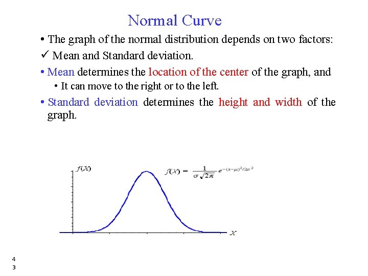
Normal Curve • The graph of the normal distribution depends on two factors: ü Mean and Standard deviation. • Mean determines the location of the center of the graph, and • It can move to the right or to the left. • Standard deviation determines the height and width of the graph. 4 3

Standard Normal Distribution (SND) • It makes life a lot easier for us if we standardize our normal curve, with a mean of zero and a standard deviation of 1 unit. • We can transform all the observations of any normal random variable X with mean μ and variance σ to a new set of observations of another normal random variable Z with mean 0 and variance 1 using the following transformation: 4 4

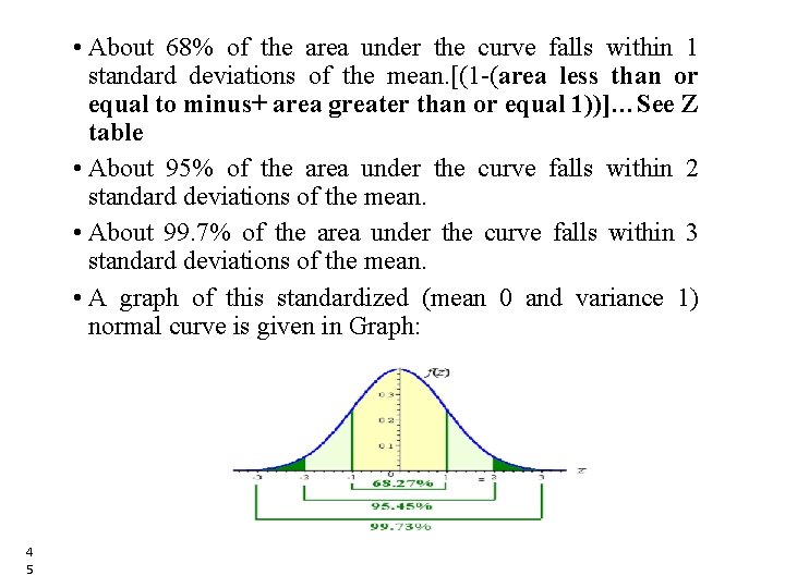
• About 68% of the area under the curve falls within 1 standard deviations of the mean. [(1 -(area less than or equal to minus+ area greater than or equal 1))]…See Z table • About 95% of the area under the curve falls within 2 standard deviations of the mean. • About 99. 7% of the area under the curve falls within 3 standard deviations of the mean. • A graph of this standardized (mean 0 and variance 1) normal curve is given in Graph: 4 5

Standard Normal Distribution (SND) • Has a published table (Z-table) • An observation from a normal distribution can be related to a SND • An observation x from a normal distribution with mean μ and SD (σ) can be related to the SND. • This is done by subtracting the mean from each observation and dividing by SD. • This is called Z-transformation 4 6

Z- transformation • If a random variable X~ N(μ , σ ) then we can transform it to a standard normal distribution with the help of Z-transformation Ø Z = X –μ σ 4 7

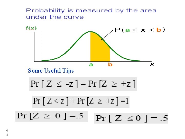
Some Useful Tips 4 8

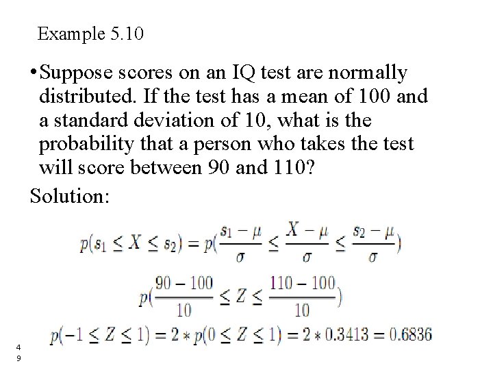
Example 5. 10 • Suppose scores on an IQ test are normally distributed. If the test has a mean of 100 and a standard deviation of 10, what is the probability that a person who takes the test will score between 90 and 110? Solution: 4 9

5 2

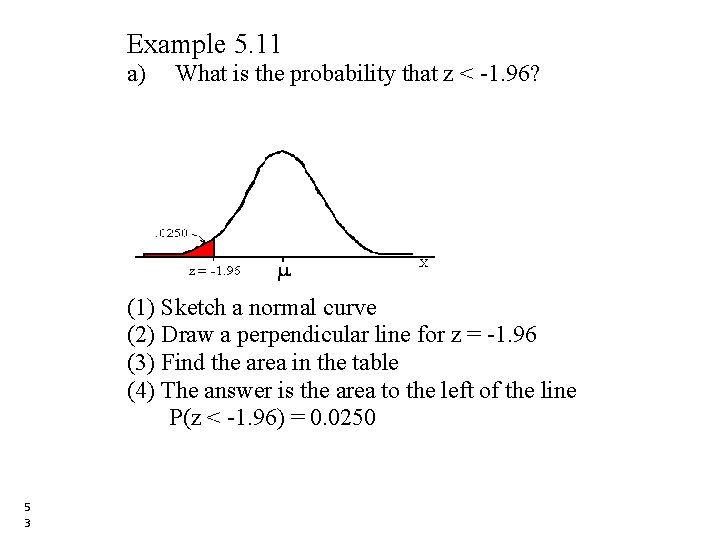
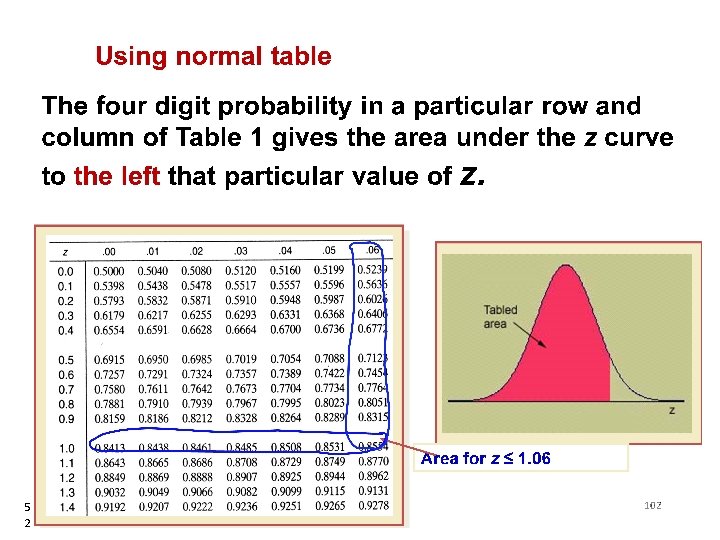
Example 5. 11 a) What is the probability that z < -1. 96? (1) Sketch a normal curve (2) Draw a perpendicular line for z = -1. 96 (3) Find the area in the table (4) The answer is the area to the left of the line P(z < -1. 96) = 0. 0250 5 3

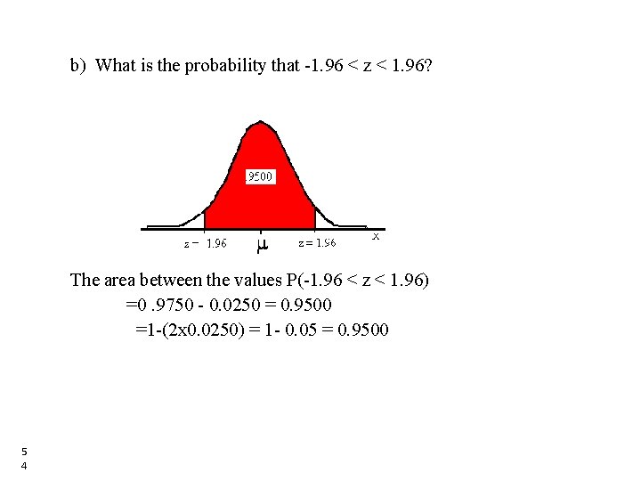
b) What is the probability that -1. 96 < z < 1. 96? The area between the values P(-1. 96 < z < 1. 96) =0. 9750 - 0. 0250 = 0. 9500 =1 -(2 x 0. 0250) = 1 - 0. 05 = 0. 9500 5 4

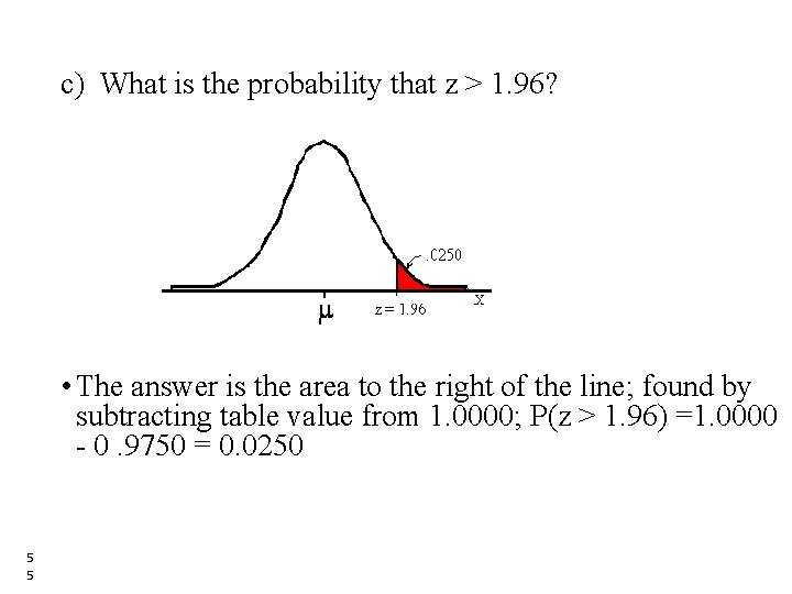
c) What is the probability that z > 1. 96? • The answer is the area to the right of the line; found by subtracting table value from 1. 0000; P(z > 1. 96) =1. 0000 - 0. 9750 = 0. 0250 5 5

Application/Uses of Normal Distribution • It’s application goes beyond describing distributions • It is used by researchers and modelers. • The major use of normal distribution is the role it plays in statistical inference. • The z score along with the t –score, is important in hypothesis testing. • It helps managers/management make decisions. 5 6

Exercise 1. Compute P(-1 ≤ Z ≤ 1. 5) Ans: 0. 7745 2. Find the area under the SND from 0 to 1. 45 Ans: 0. 4265 3. Compute P(-1. 66 < Z < 2. 85) Ans: 0. 9493 5 7

Student t-distribution 5 8 • It is often the case that one wants to calculate the size of sample needed to obtain a certain level of confidence in survey results. • Unfortunately, this calculation requires prior knowledge of the population standard deviation σ. • Realistically, σ is unknown • Often a preliminary sample will be conducted so that a reasonable estimate of this critical population parameter can be made. • If such a preliminary sample is not made, but confidence intervals for the population mean are to be constructing using an unknown σ, then the distribution known as the Student t distribution can be used.

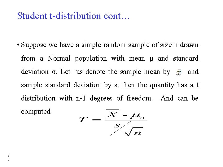
Student t-distribution cont… • Suppose we have a simple random sample of size n drawn from a Normal population with mean μ and standard deviation σ. Let us denote the sample mean by and sample standard deviation by s, then the quantity has a t distribution with n-1 degrees of freedom. And can be computed 5 9

Some properties of t-distribution • It is roughly shaped like the normal distribution, but is with less peaked in the center and with broader tails. • It has mean of zero (Symmetric around zero) • It is symmetric about the mean. • It ranges from -� to �. . • It depends on the degrees of freedom (n-1). • It Converges to the normal distribution as the sample size gets large 6 0