Probabilistic Robotics Introduction Probabilities Bayes rule Bayes filters

Probabilistic Robotics Introduction Probabilities Bayes rule Bayes filters

Probabilistic Robotics Key idea: Explicit representation of uncertainty using the calculus of probability theory • Perception = state estimation • Action = utility optimization 2
 denotes probability that proposition A is true. • •")
Axioms of Probability Theory Pr(A) denotes probability that proposition A is true. • • • 3

A Closer Look at Axiom 3 B 4

Using the Axioms 5

Discrete Random Variables • X denotes a random variable. • X can take on a countable number of values in {x 1, x 2, …, xn}. • P(X=xi), or P(xi), is the probability that the random variable X takes on value xi. • P(. ) is called probability mass function. • E. g. 6
, or")
Continuous Random Variables • X takes on values in the continuum. • p(X=x), or p(x), is a probability density function. p(x) • E. g. x 7
 = P(x, y) • If X")
Joint and Conditional Probability • P(X=x and Y=y) = P(x, y) • If X and Y are independent then P(x, y) = P(x) P(y) • P(x | y) is the probability of x given y P(x | y) = P(x, y) / P(y) P(x, y) = P(x | y) P(y) • If X and Y are independent then P(x | y) = P(x) 8
 = P(A and B) / P(B) B 0. 5 A")
Conditional Probability • P(A|B) = P(A and B) / P(B) B 0. 5 A 0. 2 Introduction to Robotics ��������� 3 ���� 9 P(A|B) = 0. 2/0. 5

Law of Total Probability, Marginals Discrete case Continuous case 10

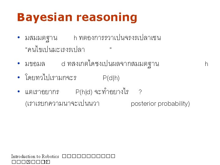
Bayes Formula 11

Bayesian reasoning “judging” one’s intuition Scenario: Prosecutor: Defendant: Suppose a crime has been committed. Blood is found at the scene for which there is no innocent explanation. It is of a blood type which is present in 1% of the population and present in the defendant. There is a 1% chance that the defendant would have the crime scene’s blood type if innocent, so there is a 99% chance that the defendant is guilty. The crime occurred in a city of 800, 000 people (suppose true). There, the blood type would be found in approximately 8, 000 people, so this evidence only provides a negligible 0. 0125% (= 1/8000) chance of guilt. Introduction to Robotics ����� 3 ���� 16

Normalization Algorithm: 17

Conditioning • Law of total probability: 18

Bayes Rule with Background Knowledge 19

Conditioning • Total probability: 20

Conditional Independence equivalent to and 21

Simple Example of State Estimation • Suppose a robot obtains measurement z • What is P(open|z)? 22
 is diagnostic. • P(z|open) is causal. • Often")
Causal vs. Diagnostic Reasoning • P(open|z) is diagnostic. • P(z|open) is causal. • Often causal knowledge is easier to obtain. count frequencies! • Bayes rule allows us to use causal knowledge: 23
 = 0. 6 P(z| open) = 0. 3 • P(open) =")
Example • P(z|open) = 0. 6 P(z| open) = 0. 3 • P(open) = P( open) = 0. 5 • z raises the probability that the door is open. 24

Combining Evidence • Suppose our robot obtains another observation z 2. • How can we integrate this new information? • More generally, how can we estimate P(x| z 1. . . zn )? 25

Recursive Bayesian Updating Markov assumption: zn is independent of z 1, . . . , zn-1 if we know x. 26
 = 0. 5 • P(open|z 1)=2/3 P(z 2|")
Example: Second Measurement • P(z 2|open) = 0. 5 • P(open|z 1)=2/3 P(z 2| open) = 0. 6 • z 2 lowers the probability that the door is open. 27

A Typical Pitfall • Two possible locations x 1 and x 2 • P(x 1)=0. 99 • P(z|x 2)=0. 09 P(z|x 1)=0. 07 28

Actions • Often the world is dynamic since • actions carried out by the robot, • actions carried out by other agents, • or just the time passing by change the world. • How can we incorporate such actions? 29

Typical Actions • The robot turns its wheels to move • The robot uses its manipulator to grasp • an object Plants grow over time… • Actions are never carried out with • absolute certainty. In contrast to measurements, actions generally increase the uncertainty. 30

Modeling Actions • To incorporate the outcome of an action u into the current “belief”, we use the conditional pdf P(x|u, x’) • This term specifies the pdf that executing u changes the state from x’ to x. 31

Example: Closing the door 32
 for u = “close door”: If the door is open,")
State Transitions P(x|u, x’) for u = “close door”: If the door is open, the action “close door” succeeds in 90% of all cases. 33

Integrating the Outcome of Actions Continuous case: Discrete case: 34

Example: The Resulting Belief 35

Bayes Filters: Framework • Given: • Stream of observations z and action data u: • Sensor model P(z|x). • Action model P(x|u, x’). • Prior probability of the system state P(x). • Wanted: • Estimate of the state X of a dynamical system. • The posterior of the state is also called Belief: 36

Markov Assumption Underlying Assumptions • Static world • Independent noise • Perfect model, no approximation errors 37

Bayes Filters z = observation u = action x = state Bayes Markov Total prob. Markov 38
,")
Bayes Filter Algorithm 1. 2. 3. 4. 5. 6. 7. 8. Algorithm Bayes_filter( Bel(x), d ): h=0 If d is a perceptual data item z then For all x do 9. Else if d is an action data item u then 10. For all x do 11. 12. Return Bel’(x) 39

Bayes Filters are Familiar! • Kalman filters • Particle filters • Hidden Markov models • Dynamic Bayesian networks • Partially Observable Markov Decision Processes (POMDPs) 40

Summary • Bayes rule allows us to compute probabilities that are hard to assess otherwise. • Under the Markov assumption, recursive Bayesian updating can be used to efficiently combine evidence. • Bayes filters are a probabilistic tool for estimating the state of dynamic systems. 41
- Slides: 41