Probabilistic Models of Cortical Computation Rajesh P N

Probabilistic Models of Cortical Computation Rajesh P. N. Rao Dept. of Computer Sci. and Engineering & Neurobio. and Behavior Program University of Washington Seattle, WA Lab website: http: //neural. cs. washington. edu November, 2004 Funding: Sloan Foundation, Packard Foundation, ONR, and NSF 1

Why Consider Probabilistic Models? Computational Reasons F Sensory measurements are typically ambiguous í E. g. Projection from 3 D to 2 D in vision F Biological sensors and processing elements are noisy F Animal’s knowledge of the world is usually incomplete There appears to be a need to be able to represent, learn, and reason about probabilities 2

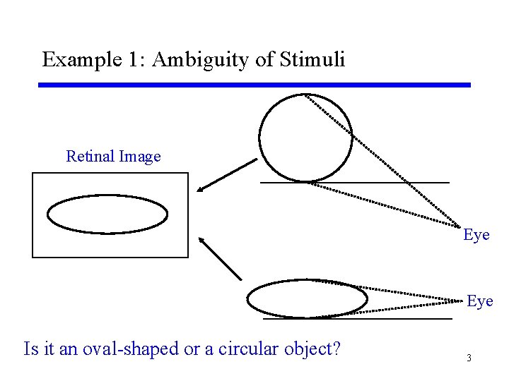
Example 1: Ambiguity of Stimuli Retinal Image Eye Is it an oval-shaped or a circular object? 3

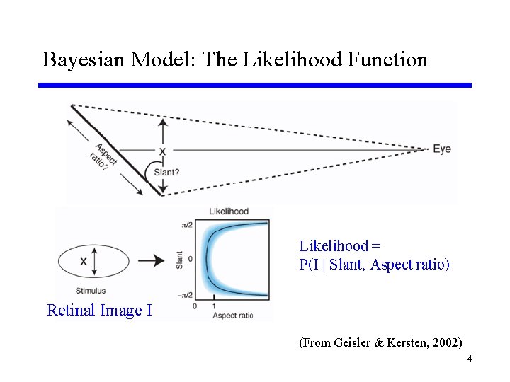
Bayesian Model: The Likelihood Function Likelihood = P(I | Slant, Aspect ratio) Retinal Image I (From Geisler & Kersten, 2002) 4

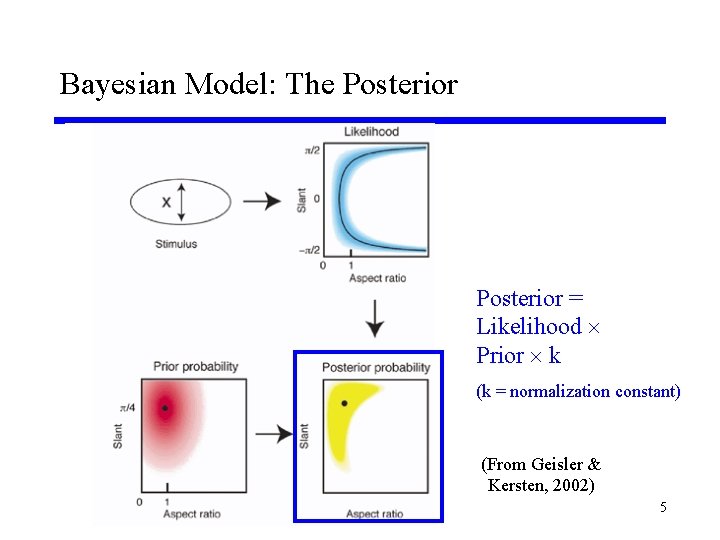
Bayesian Model: The Posterior = Likelihood Prior k (k = normalization constant) (From Geisler & Kersten, 2002) 5

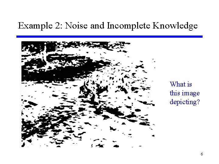
Example 2: Noise and Incomplete Knowledge What is this image depicting? 6

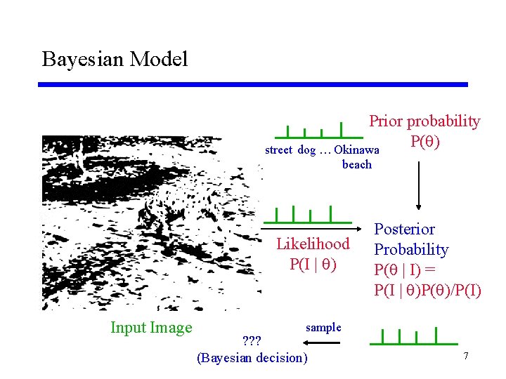
Bayesian Model street Prior probability P( ) dog … Okinawa beach Likelihood P(I | ) Input Image Posterior Probability P( | I) = P(I | )P( )/P(I) sample ? ? ? (Bayesian decision) 7

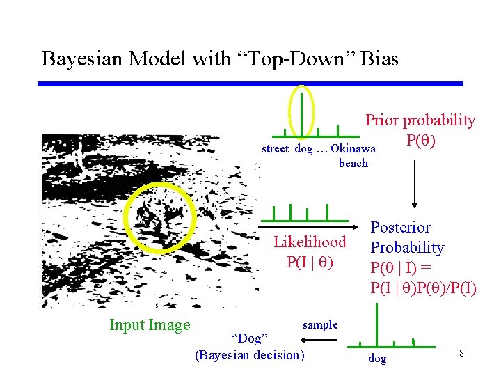
Bayesian Model with “Top-Down” Bias street Prior probability P( ) dog … Okinawa beach Likelihood P(I | ) Input Image Posterior Probability P( | I) = P(I | )P( )/P(I) sample “Dog” (Bayesian decision) dog 8

Psychophysical Evidence for Bayesian Perception F Motion from cast shadows (Kersten et al. , 1996) F Surface perception based on texture (Knill, 1998) F Inferring 3 D shape from 2 D images (Mamassian et al. , 2002) F Color perception (Bloj et al. , 1999) F Cue combination for depth perception (Jacobs, 2002) F Motion illusions (Weiss et al. , 2002) F Motor Control (Körding and Wolpert, 2004) 9

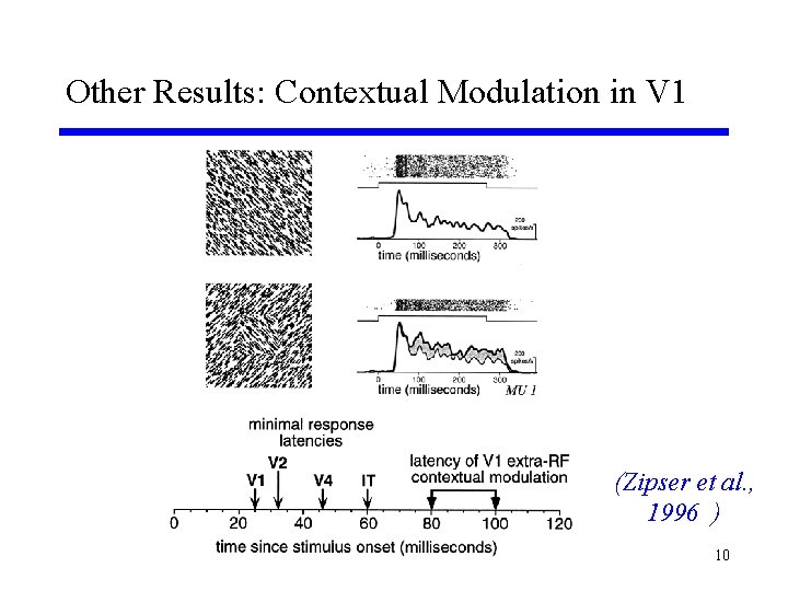
Other Results: Contextual Modulation in V 1 (Zipser et al. , 1996 ) 10

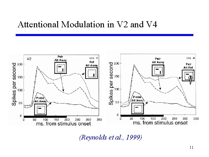
Attentional Modulation in V 2 and V 4 (Reynolds et al. , 1999) 11

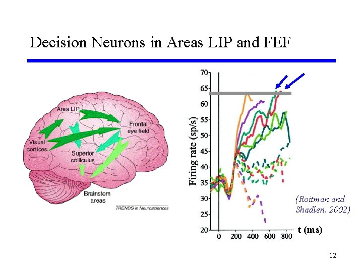
Decision Neurons in Areas LIP and FEF (Roitman and Shadlen, 2002) t (ms) 12

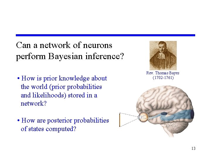
Can a network of neurons perform Bayesian inference? • How is prior knowledge about the world (prior probabilities and likelihoods) stored in a network? Rev. Thomas Bayes (1702 -1761) • How are posterior probabilities of states computed? 13

Generative Models for Bayesian Inference F Fundamental Idea: Inputs received by an organism are caused by external “states” of the world (hidden “causes”) F Goal: Estimate the probability of these causes (or states or “interpretations”) based on the inputs received thus far 14

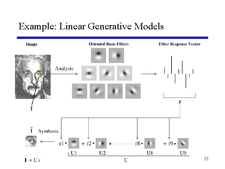
Example: Linear Generative Models 15

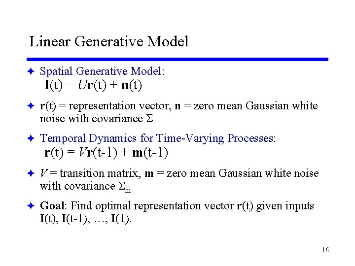
Linear Generative Model F Spatial Generative Model: I(t) = Ur(t) + n(t) F r(t) = representation vector, n = zero mean Gaussian white noise with covariance F Temporal Dynamics for Time-Varying Processes: r(t) = Vr(t-1) + m(t-1) F V = transition matrix, m = zero mean Gaussian white noise with covariance m F Goal: Find optimal representation vector r(t) given inputs I(t), I(t-1), …, I(1). 16

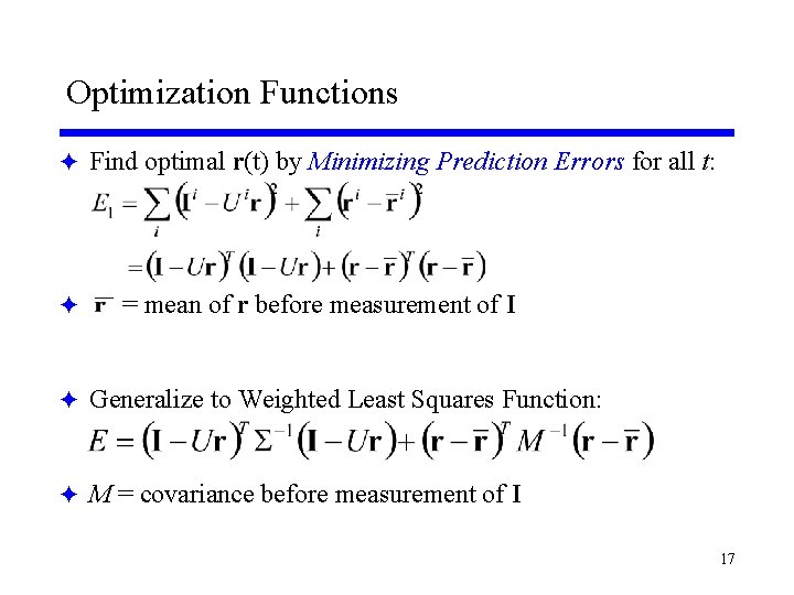
Optimization Functions F Find optimal r(t) by Minimizing Prediction Errors for all t: F = mean of r before measurement of I F Generalize to Weighted Least Squares Function: F M = covariance before measurement of I 17

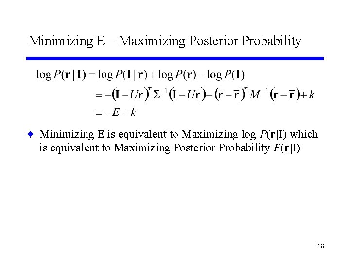
Minimizing E = Maximizing Posterior Probability F Minimizing E is equivalent to Maximizing log P(r|I) which is equivalent to Maximizing Posterior Probability P(r|I) 18

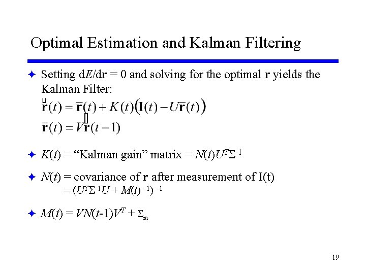
Optimal Estimation and Kalman Filtering F Setting d. E/dr = 0 and solving for the optimal r yields the Kalman Filter: F K(t) = “Kalman gain” matrix = N(t)UT -1 F N(t) = covariance of r after measurement of I(t) = (UT -1 U + M(t) -1 F M(t) = VN(t-1)VT + m 19

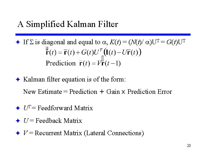
A Simplified Kalman Filter F If is diagonal and equal to , K(t) = (N(t)/ )UT = G(t)UT F Kalman filter equation is of the form: New Estimate = Prediction + Gain x Prediction Error F UT = Feedforward Matrix F U = Feedback Matrix F V = Recurrent Matrix (Lateral Connections) 20

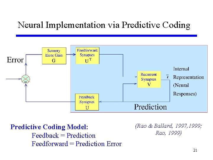
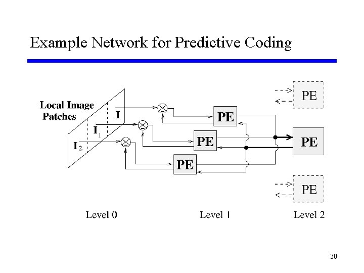
Neural Implementation via Predictive Coding Model: Feedback = Prediction Feedforward = Prediction Error (Rao & Ballard, 1997, 1999; Rao, 1999) 21

Clues from Cortical Anatomy Higher Area Lower Area 22

Hierarchical Organization of the Visual Cortex Higher Lower 23

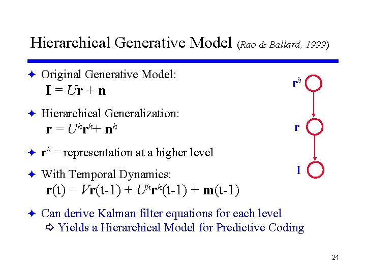
Hierarchical Generative Model (Rao & Ballard, 1999) F Original Generative Model: I = Ur + n rh F Hierarchical Generalization: r = Uhrh+ nh r F rh = representation at a higher level F With Temporal Dynamics: I r(t) = Vr(t-1) + Uhrh(t-1) + m(t-1) F Can derive Kalman filter equations for each level í Yields a Hierarchical Model for Predictive Coding 24

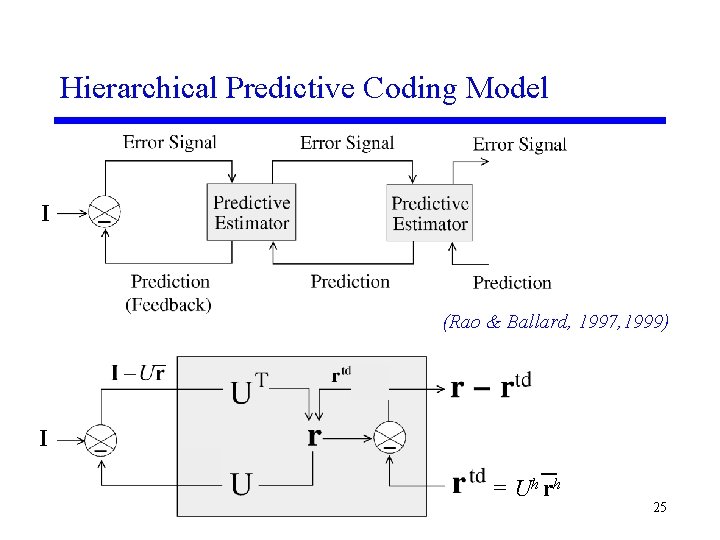
Hierarchical Predictive Coding Model I (Rao & Ballard, 1997, 1999) I = Uh rh 25

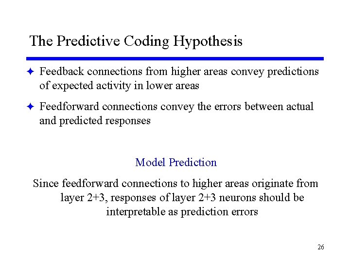
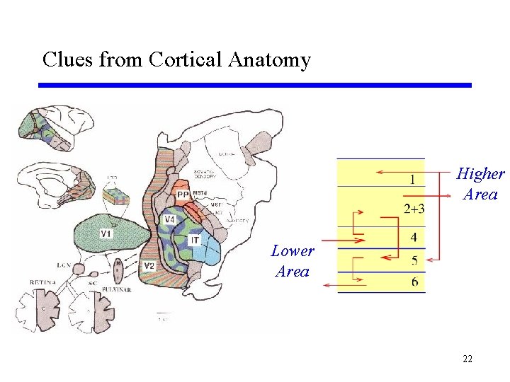
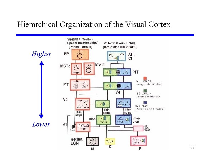
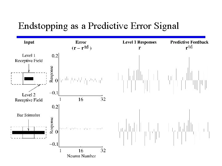
The Predictive Coding Hypothesis F Feedback connections from higher areas convey predictions of expected activity in lower areas F Feedforward connections convey the errors between actual and predicted responses Model Prediction Since feedforward connections to higher areas originate from layer 2+3, responses of layer 2+3 neurons should be interpretable as prediction errors 26

Results from the Classic Studies of Hubel and Weisel (1960 s) 27

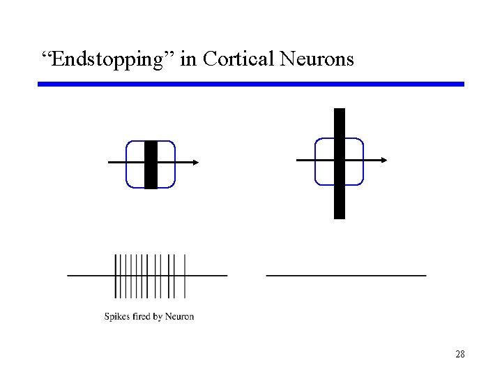
“Endstopping” in Cortical Neurons 28

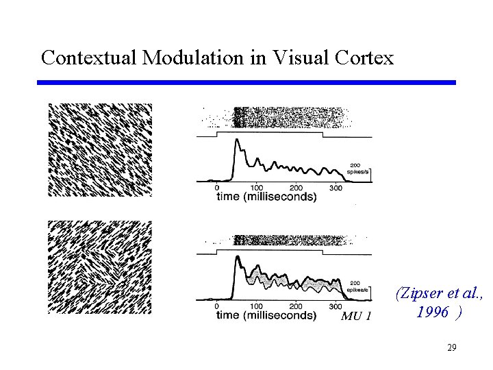
Contextual Modulation in Visual Cortex (Zipser et al. , 1996 ) 29

Example Network for Predictive Coding 30

Natural Images used for Training 31

Synaptic Weights after Learning 32

Endstopping as a Predictive Error Signal 33

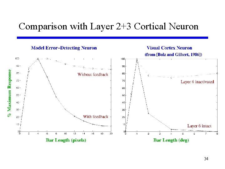
Comparison with Layer 2+3 Cortical Neuron 34

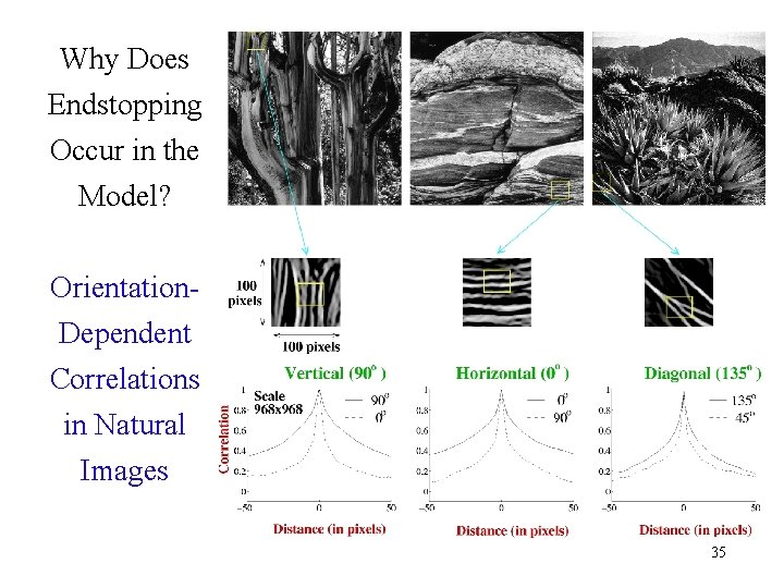
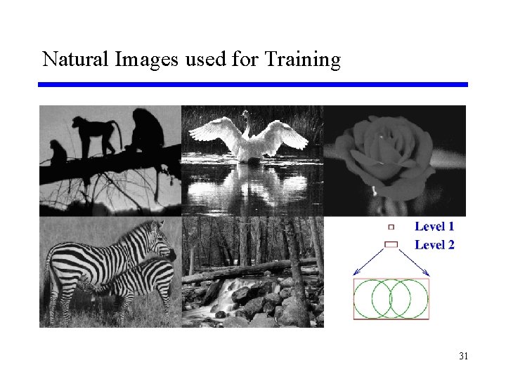
Why Does Endstopping Occur in the Model? Orientation. Dependent Correlations in Natural Images 35

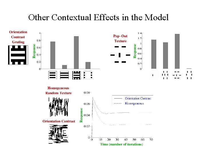
Other Contextual Effects in the Model 36

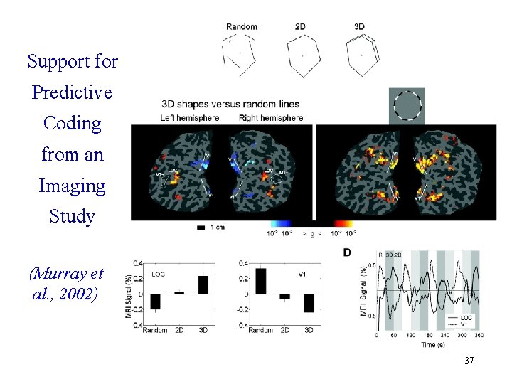
Support for Predictive Coding from an Imaging Study (Murray et al. , 2002) 37

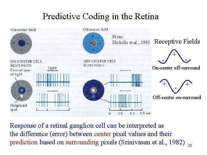
Predictive Coding in the Retina From: Nicholls et al. , 1992 Receptive Fields - + - On-center off-surround + - + Off-center on-surround Response of a retinal ganglion cell can be interpreted as the difference (error) between center pixel values and their prediction based on surrounding pixels (Srinivasan et al. , 1982) 38

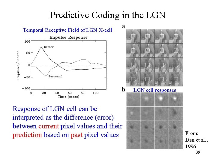
Predictive Coding in the LGN Temporal Receptive Field of LGN X-cell LGN cell responses Response of LGN cell can be interpreted as the difference (error) between current pixel values and their prediction based on past pixel values From: Dan et al. , 1996 39

Summary for Part I F Computational and experimental studies point to the need for probabilistic models of brain function F Probabilistic models typically rely on generative models of sensory (and motor) processes F We examined a simple linear generative model and its hierarchical generalization í Bayesian inference via Kalman filtering í Neural implementation allows Hierarchical Predictive Coding ç Feedback connections convey predictions ç Feedforward connections convey errors in prediction í Hierarchical predictive coding explains endstopping and other contextual surround effects based on natural image statistics 40

Break Questions to Ponder over: 1. Can we go beyond linear generative models and Gaussian distributions? 2. Can a neural population encode an entire probability distribution rather than simply the mean or mode? 41

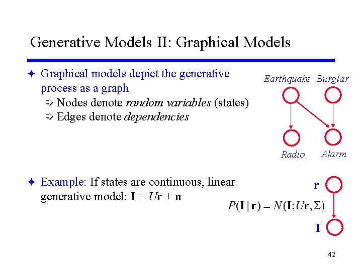
Generative Models II: Graphical Models F Graphical models depict the generative process as a graph í Nodes denote random variables (states) í Edges denote dependencies Earthquake Burglar Alarm Radio F Example: If states are continuous, linear generative model: I = Ur + n r I 42

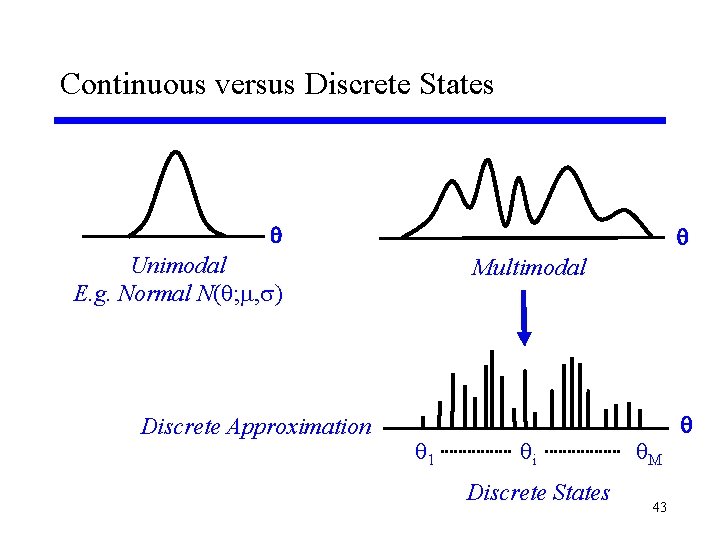
Continuous versus Discrete States Unimodal E. g. Normal N( ; , ) Discrete Approximation Multimodal 1 i Discrete States M 43

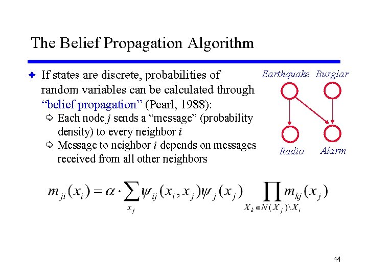
The Belief Propagation Algorithm F If states are discrete, probabilities of Earthquake Burglar random variables can be calculated through “belief propagation” (Pearl, 1988): í Each node j sends a “message” (probability density) to every neighbor i í Message to neighbor i depends on messages received from all other neighbors Radio Alarm 44

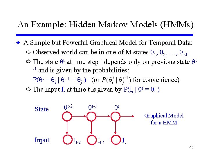
An Example: Hidden Markov Models (HMMs) F A Simple but Powerful Graphical Model for Temporal Data: í Observed world can be in one of M states 1, 2, …, M í The state t at time step t depends only on previous state t -1 and is given by the probabilities: P( t = i | t-1 = j ) (or for convenience) í The input It at time t is given by P(It | t = j ) State Input t-2 t-1 t Graphical Model for a HMM It-2 It-1 It 45

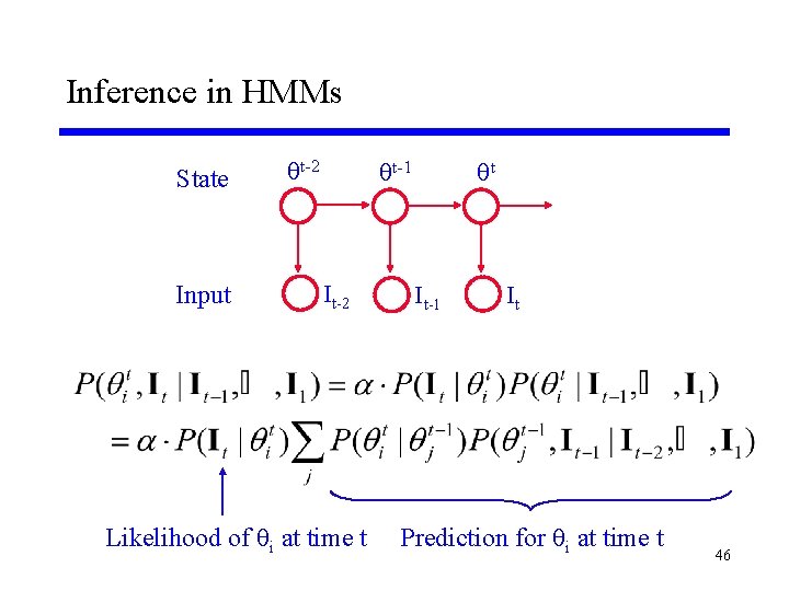
Inference in HMMs State Input t-2 t-1 It-2 Likelihood of i at time t t It-1 It Prediction for i at time t 46

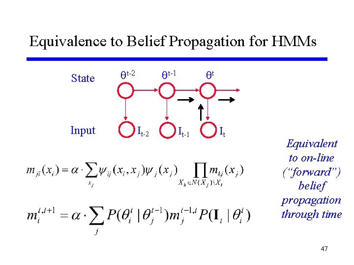
Equivalence to Belief Propagation for HMMs State Input t-2 t-1 It-2 t It-1 It Equivalent to on-line (“forward”) belief propagation through time 47

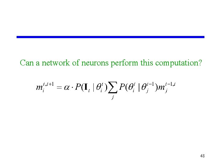
Can a network of neurons perform this computation? 48

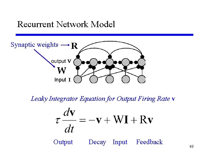
Recurrent Network Model Synaptic weights R Input I Leaky Integrator Equation for Output Firing Rate v Output Decay Input Feedback 49

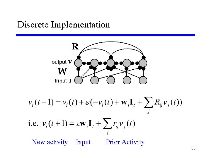
Discrete Implementation R Input I New activity Input Prior Activity 50

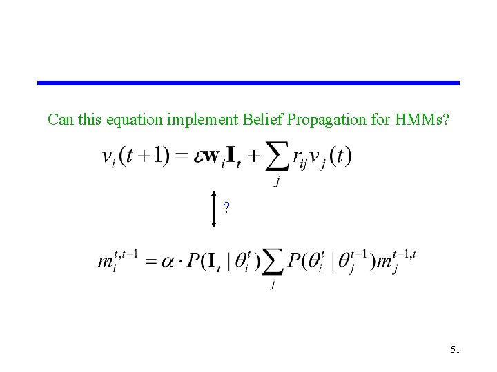
Can this equation implement Belief Propagation for HMMs? ? 51

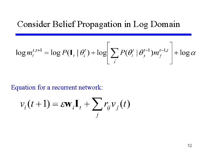
Consider Belief Propagation in Log Domain Equation for a recurrent network: 52

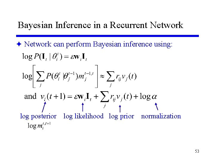
Bayesian Inference in a Recurrent Network F Network can perform Bayesian inference using: log posterior log likelihood log prior normalization 53

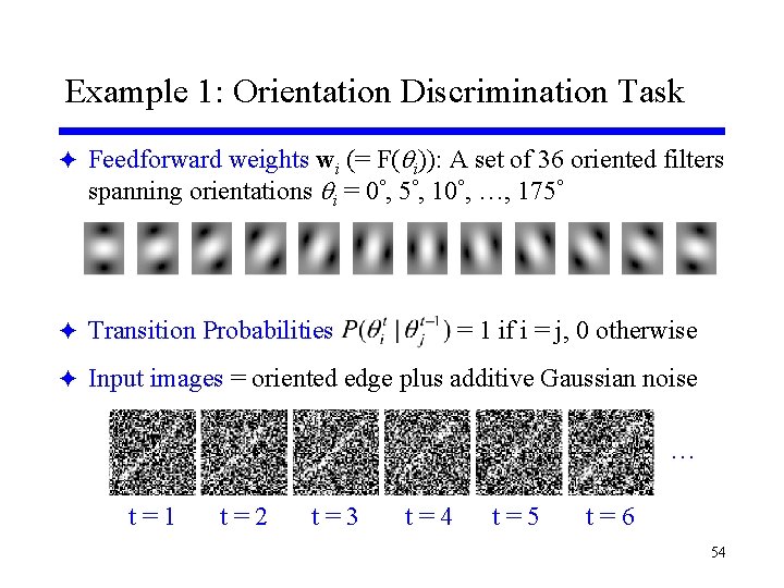
Example 1: Orientation Discrimination Task F Feedforward weights wi (= F( i)): A set of 36 oriented filters spanning orientations i = 0°, 5°, 10°, …, 175° F Transition Probabilities = 1 if i = j, 0 otherwise F Input images = oriented edge plus additive Gaussian noise … t=1 t=2 t=3 t=4 t=5 t=6 54

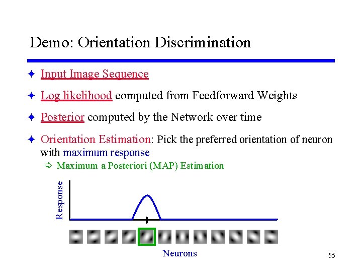
Demo: Orientation Discrimination F Input Image Sequence F Log likelihood computed from Feedforward Weights F Posterior computed by the Network over time F Orientation Estimation: Pick the preferred orientation of neuron with maximum response Response í Maximum a Posteriori (MAP) Estimation Neurons 55

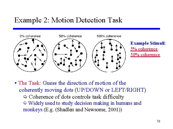
Example 2: Motion Detection Task Example Stimuli: 5% coherence 50% coherence • The Task: Guess the direction of motion of the coherently moving dots (UP/DOWN or LEFT/RIGHT) í Coherence of dots controls task difficulty í Widely used to study decision making in humans and monkeys (E. g. (Shadlen and Newsome, 2001)) 56

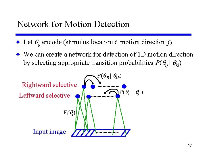
Network for Motion Detection F Let ij encode (stimulus location i, motion direction j) F We can create a network for detection of 1 D motion direction by selecting appropriate transition probabilities P( ij | kl) P( i. R | k. R) Rightward selective Leftward selective P( k. L | j. L) F( i) Input image 57

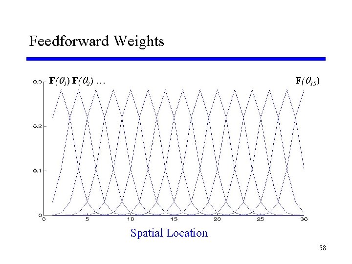
Feedforward Weights F( 1) F( 2) … F( 15) Spatial Location 58

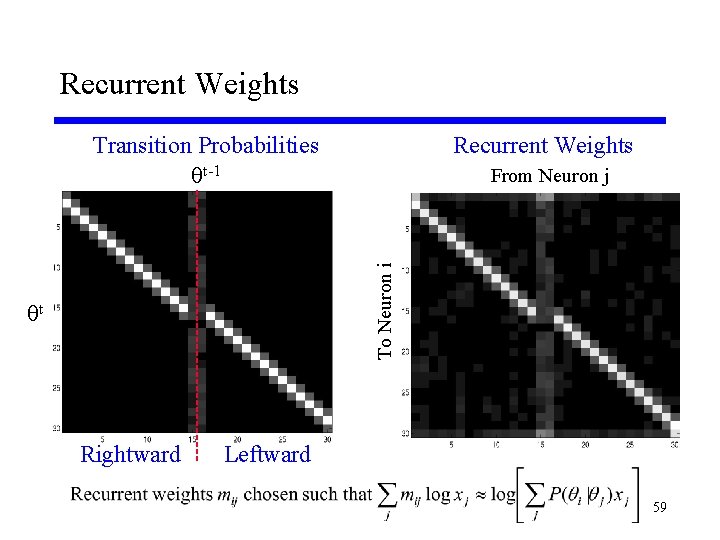
Recurrent Weights Transition Probabilities t-1 Recurrent Weights To Neuron i From Neuron j t Rightward Leftward 59

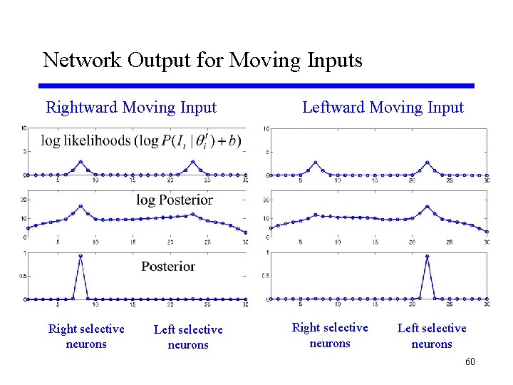
Network Output for Moving Inputs Rightward Moving Input Right selective neurons Leftward Moving Input Right selective neurons Left selective neurons 60

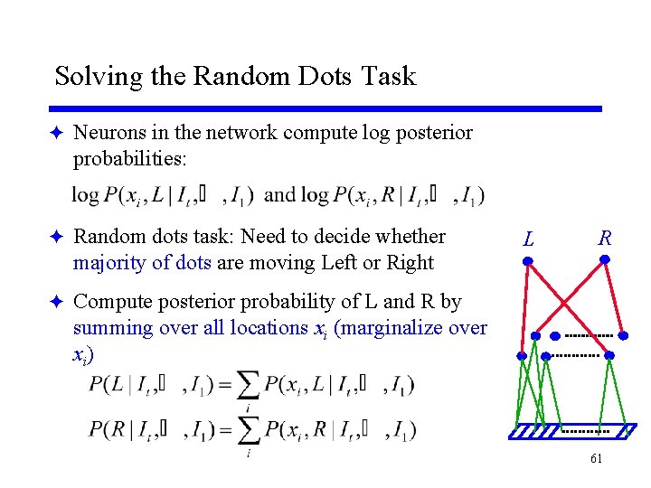
Solving the Random Dots Task F Neurons in the network compute log posterior probabilities: F Random dots task: Need to decide whether majority of dots are moving Left or Right L R F Compute posterior probability of L and R by summing over all locations xi (marginalize over x i) 61

Probabilistic Motion Detection in a Model Network F Demo 1: Activities in a model network for noisy motion í Activities represent posterior probabilities of left/rightward motion F Demo 2: Activities of model “decision” neurons í Decision neurons sum up log posterior probabilities over time í Solid line = Leftward motion, Dotted line = Rightward motion F Demo 3: Effect of making the stimulus more noisy í Longer decision times for noisier stimuli 62

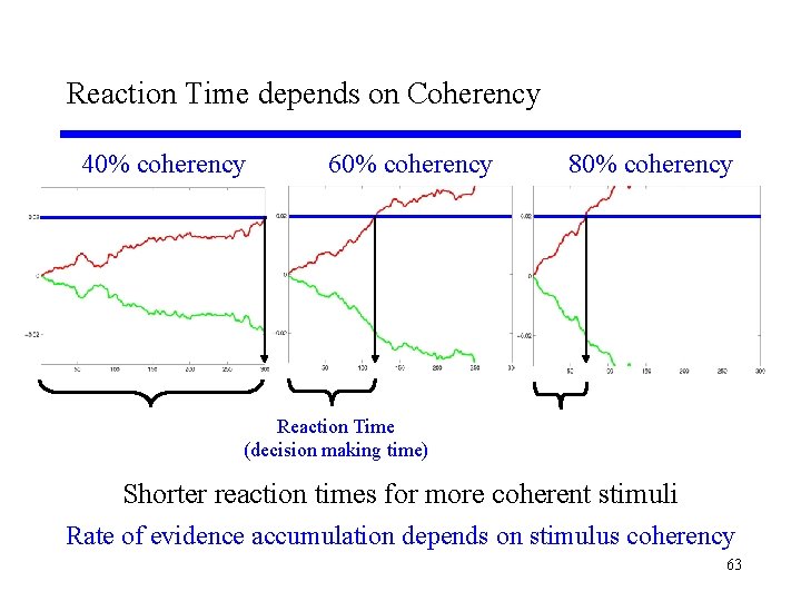
Reaction Time depends on Coherency 40% coherency 60% coherency 80% coherency Reaction Time (decision making time) Shorter reaction times for more coherent stimuli Rate of evidence accumulation depends on stimulus coherency 63

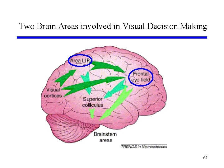
Two Brain Areas involved in Visual Decision Making 64

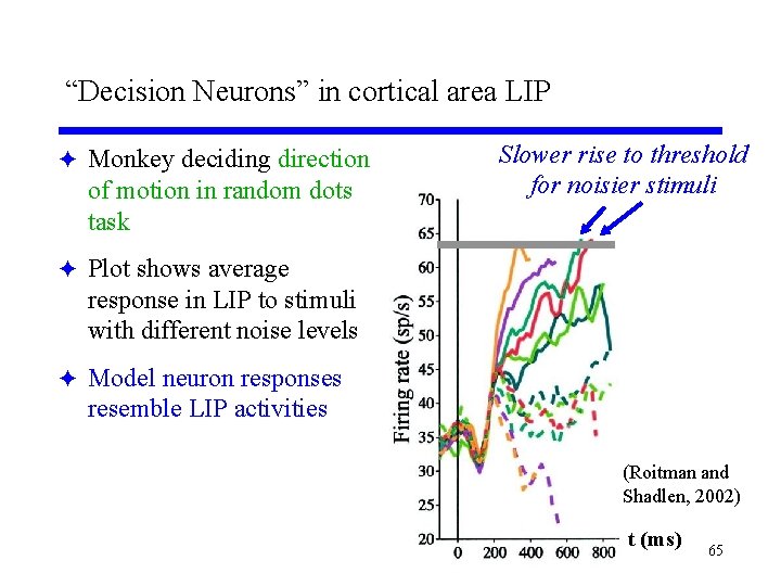
“Decision Neurons” in cortical area LIP F Monkey deciding direction of motion in random dots task Slower rise to threshold for noisier stimuli F Plot shows average response in LIP to stimuli with different noise levels F Model neuron responses resemble LIP activities (Roitman and Shadlen, 2002) t (ms) 65

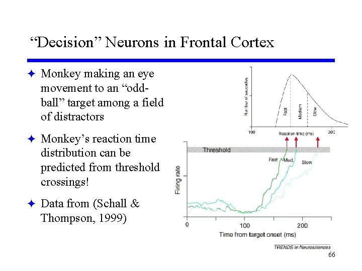
“Decision” Neurons in Frontal Cortex F Monkey making an eye movement to an “oddball” target among a field of distractors F Monkey’s reaction time distribution can be predicted from threshold crossings! F Data from (Schall & Thompson, 1999) 66

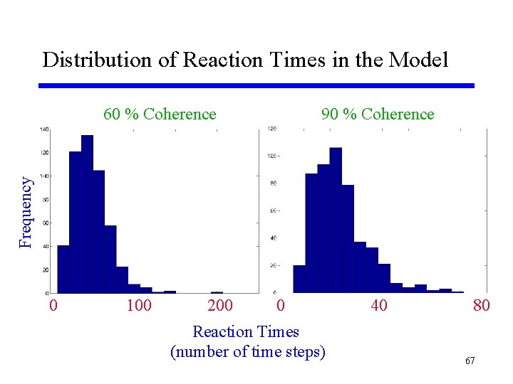
Distribution of Reaction Times in the Model 90 % Coherence Frequency 60 % Coherence 0 100 200 0 Reaction Times (number of time steps) 40 80 67

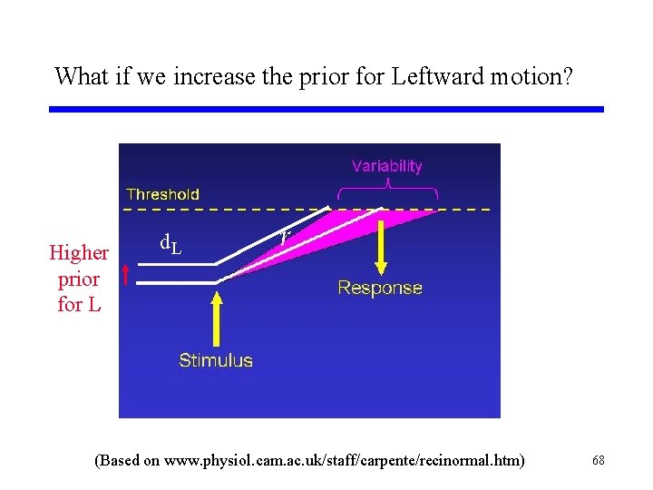
What if we increase the prior for Leftward motion? Higher prior for L d. L (Based on www. physiol. cam. ac. uk/staff/carpente/recinormal. htm) 68

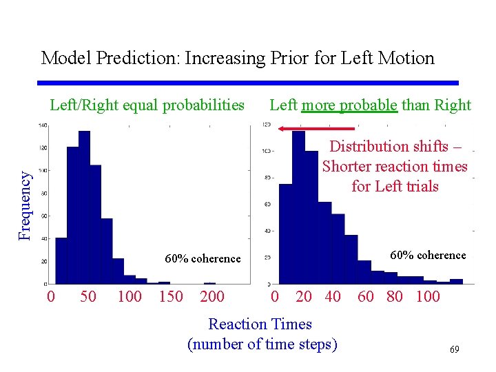
Model Prediction: Increasing Prior for Left Motion Left/Right equal probabilities Left more probable than Right Frequency Distribution shifts – Shorter reaction times for Left trials 60% coherence 0 50 100 150 200 0 20 40 Reaction Times (number of time steps) 60 80 100 69

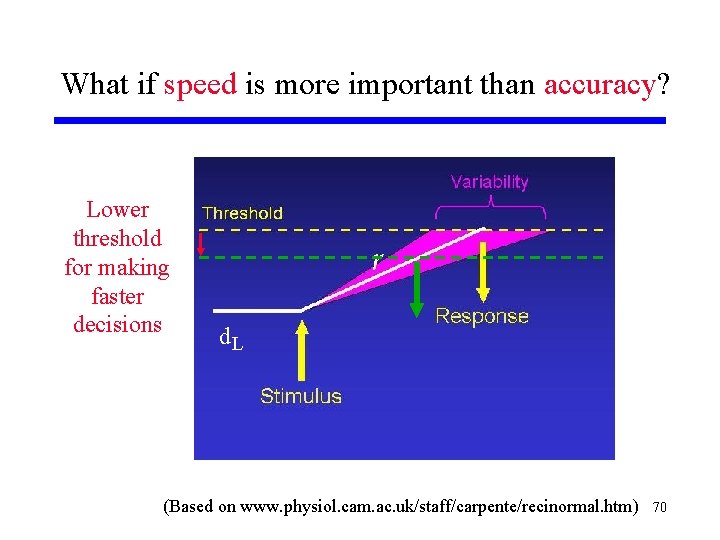
What if speed is more important than accuracy? Lower threshold for making faster decisions d. L (Based on www. physiol. cam. ac. uk/staff/carpente/recinormal. htm) 70

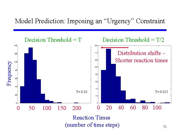
Model Prediction: Imposing an “Urgency” Constraint Decision Threshold = T/2 Frequency Distribution shifts – Shorter reaction times T= 0. 03 0 50 100 150 200 T= 0. 015 0 20 40 Reaction Times (number of time steps) 60 80 100 71

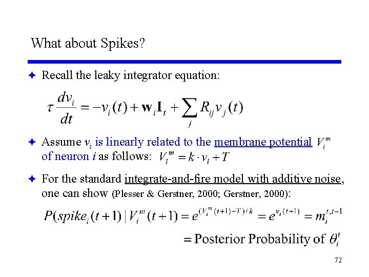
What about Spikes? F Recall the leaky integrator equation: F Assume vi is linearly related to the membrane potential of neuron i as follows: F For the standard integrate-and-fire model with additive noise, one can show (Plesser & Gerstner, 2000; Gerstner, 2000): 72

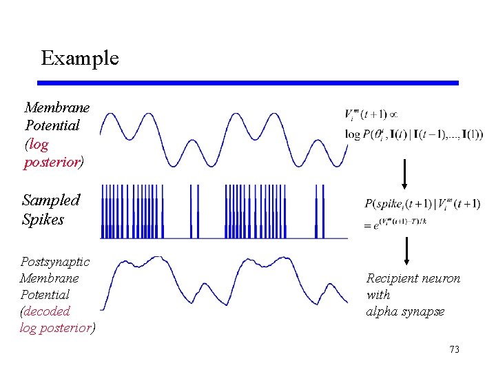
Example Membrane Potential (log posterior) Sampled Spikes Postsynaptic Membrane Potential (decoded log posterior) Recipient neuron with alpha synapse 73

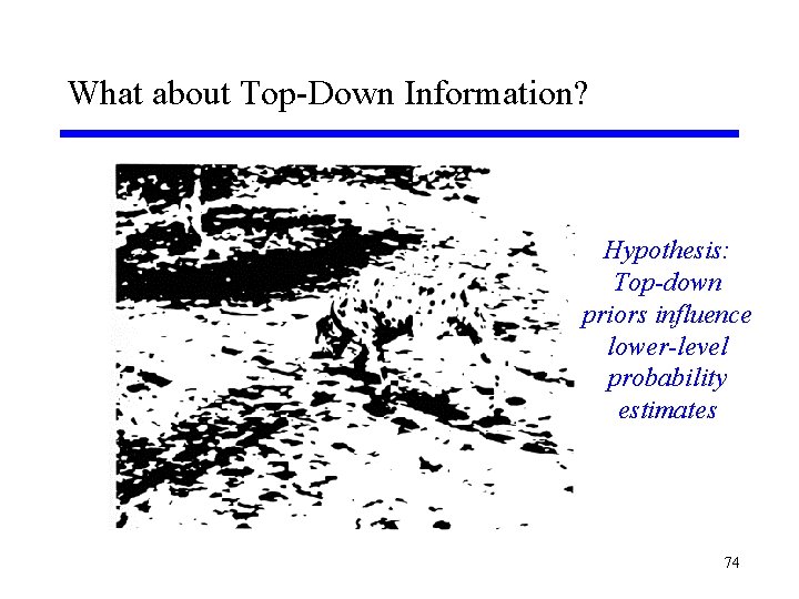
What about Top-Down Information? Hypothesis: Top-down priors influence lower-level probability estimates 74

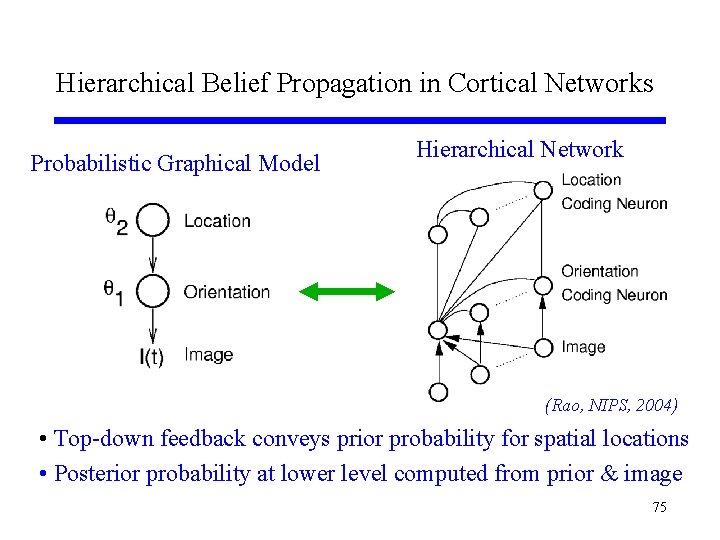
Hierarchical Belief Propagation in Cortical Networks Probabilistic Graphical Model Hierarchical Network (Rao, NIPS, 2004) • Top-down feedback conveys prior probability for spatial locations • Posterior probability at lower level computed from prior & image 75

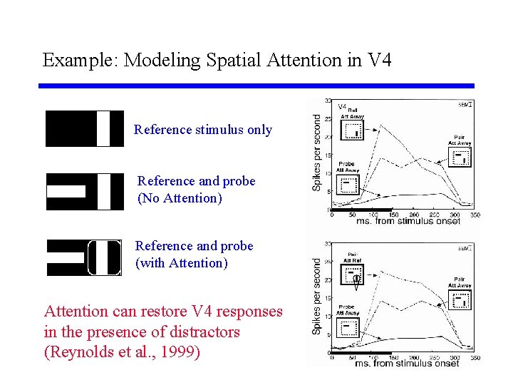
Example: Modeling Spatial Attention in V 4 Reference stimulus only Reference and probe (No Attention) Reference and probe (with Attention) Attention can restore V 4 responses in the presence of distractors (Reynolds et al. , 1999) 76

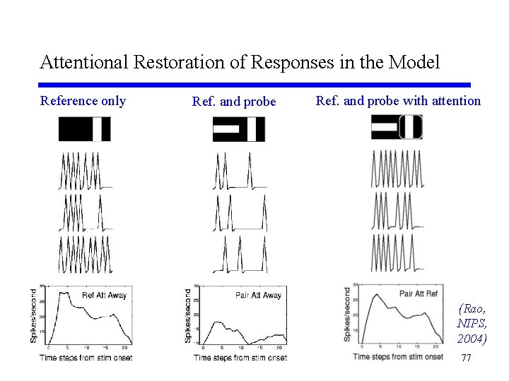
Attentional Restoration of Responses in the Model Reference only Ref. and probe with attention (Rao, NIPS, 2004) 77

Related Work on Probabilistic Models F Linear Generative Model í Sparse Coding Models (Oshausen & Field, 1996; 1997) í ICA (Bell & Sejnowski, 1997) F Hierarchical Model í Mac. Kay, 1956; Mumford, 1992; Kawato et al. , 1993; Dayan et al. , 1995; Lee & Mumford, 2003; Friston, 2003; Hawkins, 2004 F Encoding Uncertainty and Belief Propagation with Neurons í Anderson & Van Essen, 1994; Zemel et al. , 1998; Pouget et al. , 2000; Deneve, NIPS, 2004; Yu & Dayan, NIPS, 2004; Zemel et al. , NIPS, 2004 78

Summary and Conclusions (“Posterior” for this lecture) F There is growing evidence that the brain utilizes probabilistic principles such as Bayesian inference F This lecture explored two neural models for Bayesian inference: í Predictive Coding: Feedback connections convey predictions while feedforward connections carry errors í Belief Propagation: The membrane potential encodes log posterior probability via belief propagation; spiking probability is equal to posterior probability of the state encoded by the neuron F Some broad predictions of the models: í Cortical architecture implements a graphical model of the sensory (and motor) environment í Cortical networks perform hierarchical Bayesian inference í Corticocortical feedback conveys predictions or prior probabilities 79

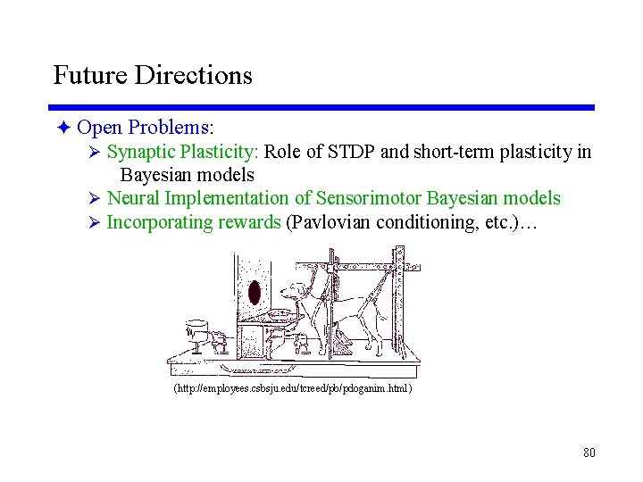
Future Directions F Open Problems: Ø Synaptic Plasticity: Role of STDP and short-term plasticity in Bayesian models Ø Neural Implementation of Sensorimotor Bayesian models Ø Incorporating rewards (Pavlovian conditioning, etc. )… (http: //employees. csbsju. edu/tcreed/pb/pdoganim. html) 80