PROBABILISTIC AND DIFFERENTIABLE PROGRAMMING V 7 Automatic Differentiation
PROBABILISTIC AND DIFFERENTIABLE PROGRAMMING V 7: Automatic Differentiation (AD) Özgür L. Özçep Universität zu Lübeck Institut für Informationssysteme
Today‘s Agenda 2

WHY YOU NEED AD 3
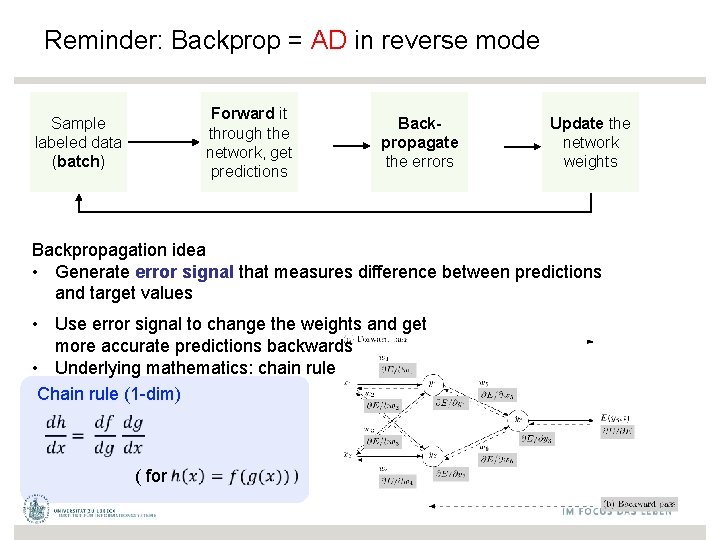
Reminder: Backprop = AD in reverse mode Forward it through the network, get predictions Sample labeled data (batch) Backpropagate the errors Update the network weights Backpropagation idea • Generate error signal that measures difference between predictions and target values • Use error signal to change the weights and get more accurate predictions backwards • Underlying mathematics: chain rule Chain rule (1 -dim) ( for
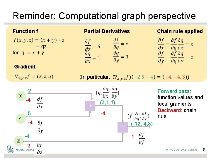
Reminder: Computational graph perspective Function f Chain rule applied Partial Derivatives Gradient (In particular: x y z -2 -4 + -4 * (-12, -4, 3) 1 -4 3 (3, 1, 1) -4 5 Forward pass: function values and local gradients Backward: chain rule 5

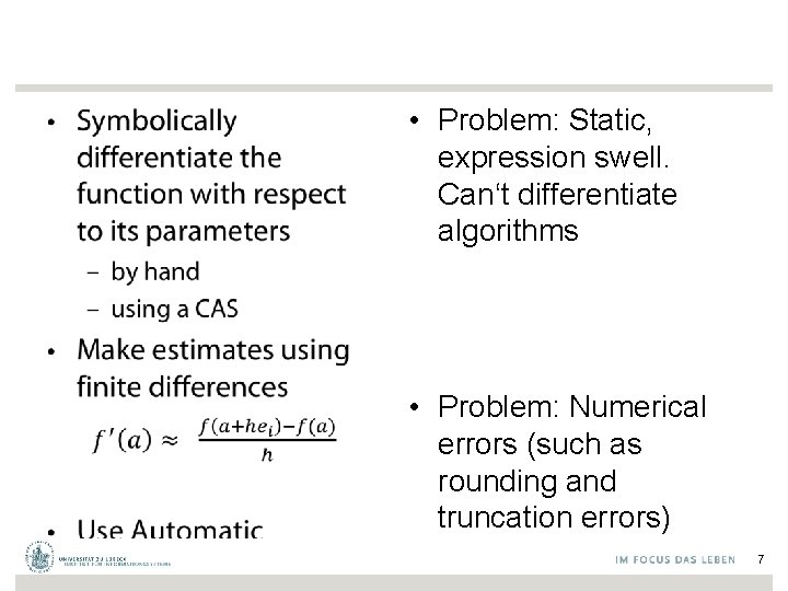
• • Problem: Static, expression swell. Can‘t differentiate algorithms • Problem: Numerical errors (such as rounding and truncation errors) 7
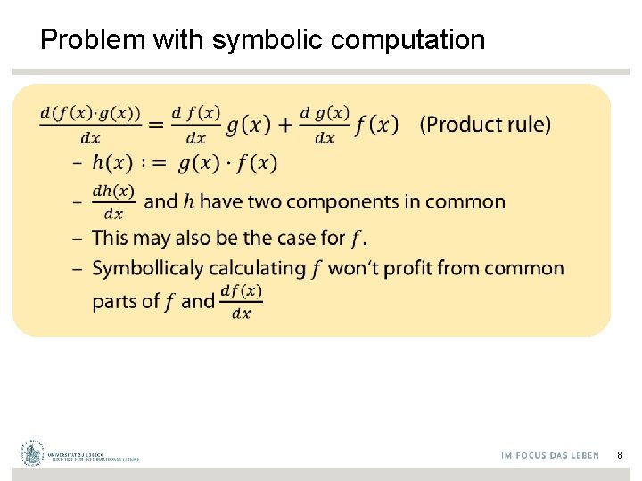
Problem with symbolic computation 8
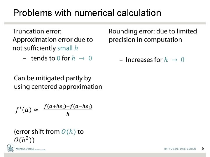
Problems with numerical calculation • • 9
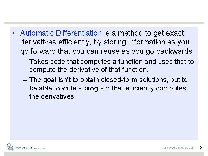
• Automatic Differentiation is a method to get exact derivatives efficiently, by storing information as you go forward that you can reuse as you go backwards. – Takes code that computes a function and uses that to compute the derivative of that function. – The goal isn’t to obtain closed-form solutions, but to be able to write a program that efficiently computes the derivatives. 10
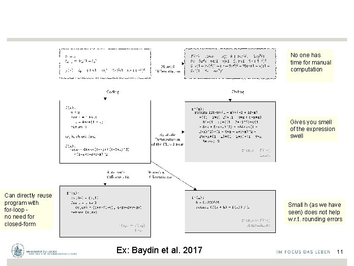
No one has time for manual computation Gives you smell of the expression swell Can directly reuse program with for-loop - no need for closed-form Small h (as we have seen) does not help w. r. t. rounding errors Ex: Baydin et al. 2017 11
AUTOMATIZATION 12
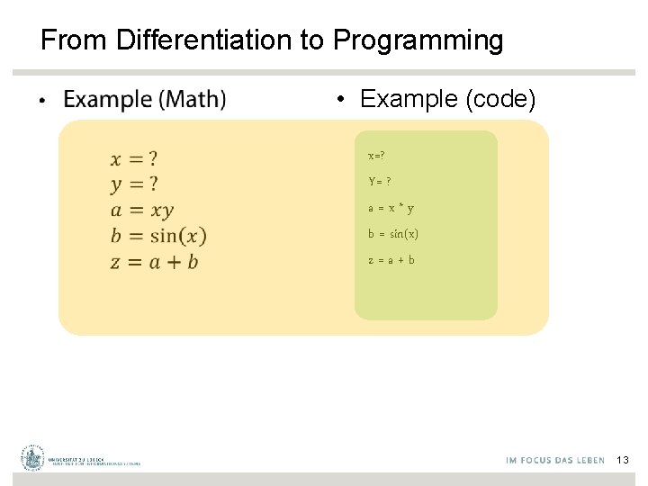
From Differentiation to Programming • • Example (code) x=? Y= ? a=x*y b = sin(x) z=a+b 13
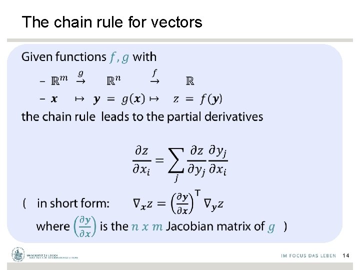
The chain rule for vectors • 14
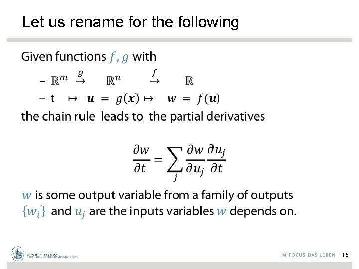
Let us rename for the following • 15
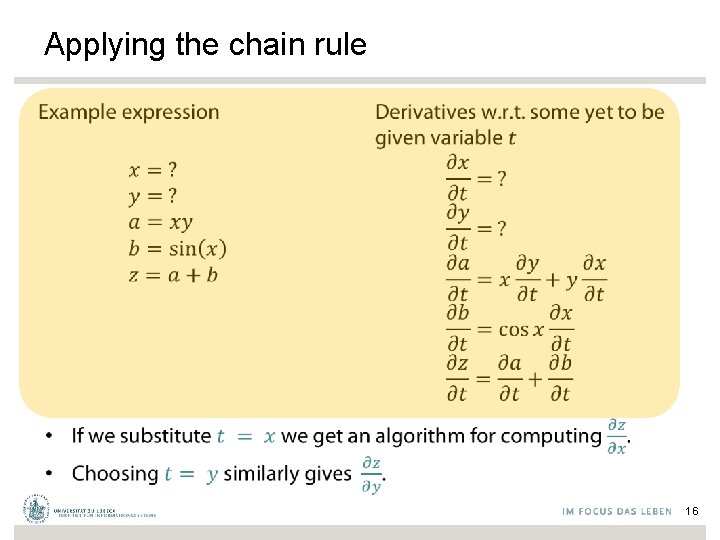
Applying the chain rule • • 16
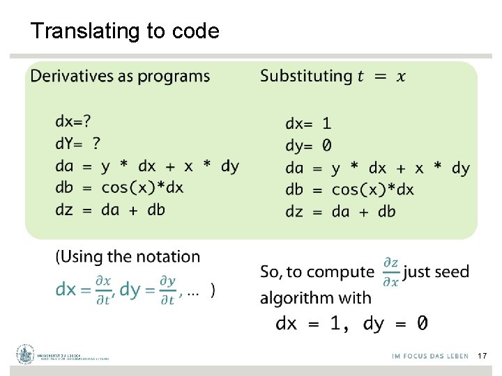
Translating to code • • 17
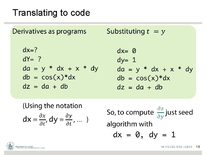
Translating to code • • 18
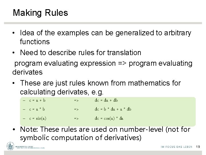
Making Rules • Idea of the examples can be generalized to arbitrary functions • Need to describe rules for translation program evaluating expression => program evaluating derivates • These are just rules known from mathematics for calculating derivates, e. g. – c=a+b – c=a*b – c = sin(a) => => => dc = da + db dc = b * da + a * db dc = cos(a) * da • Note: These rules are used on number-level (not for symbolic computation of derivatives) 19
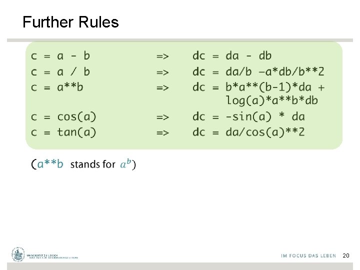
Further Rules • 20

FORWARD MODE 21
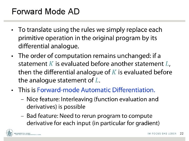
Forward Mode AD • 22
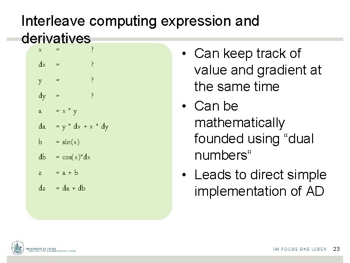
Interleave computing expression and derivatives x dx y dy a da b db z dz = ? = ? =x*y = y * dx + x * dy = sin(x) = cos(x)*dx =a+b = da + db • Can keep track of value and gradient at the same time • Can be mathematically founded using “dual numbers“ • Leads to direct simplementation of AD 23
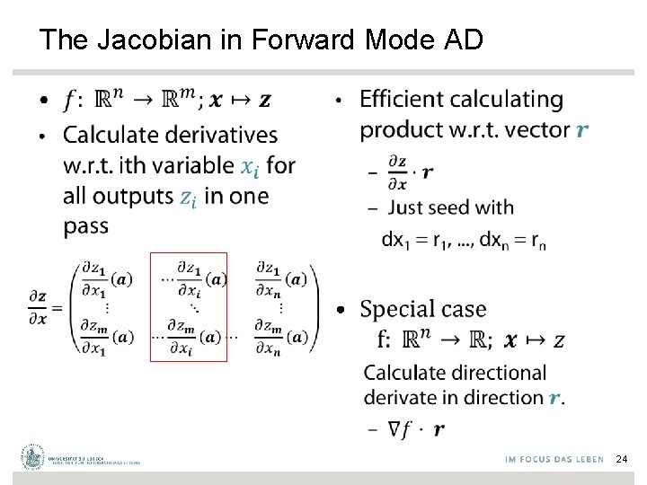
The Jacobian in Forward Mode AD • • 24
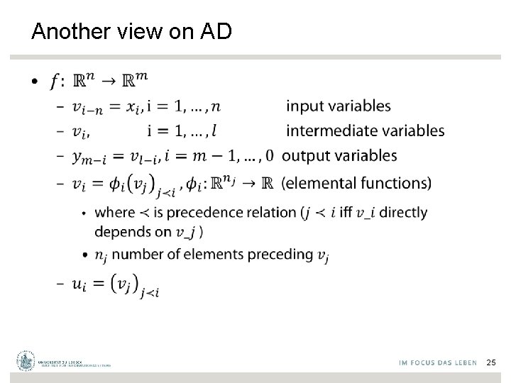
Another view on AD • 25
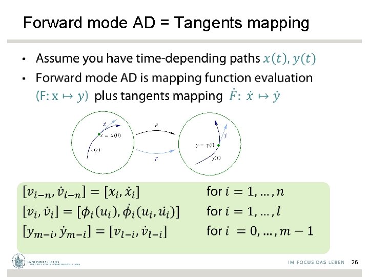
Forward mode AD = Tangents mapping • 26
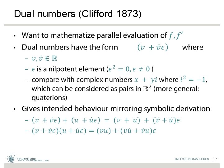
Dual numbers (Clifford 1873) • 27
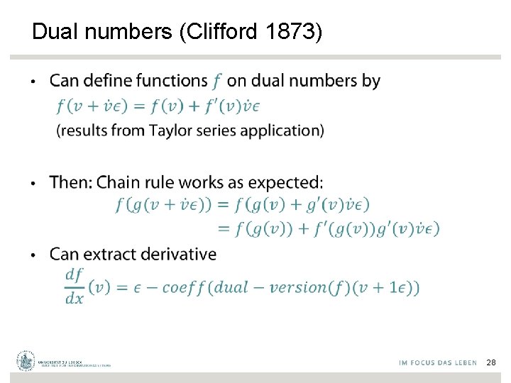
Dual numbers (Clifford 1873) • 28
REVERSE MODE 29
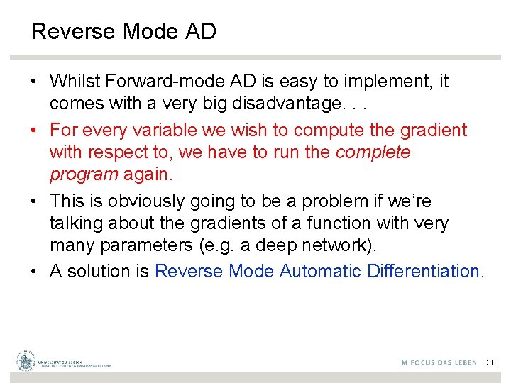
Reverse Mode AD • Whilst Forward-mode AD is easy to implement, it comes with a very big disadvantage. . . • For every variable we wish to compute the gradient with respect to, we have to run the complete program again. • This is obviously going to be a problem if we’re talking about the gradients of a function with very many parameters (e. g. a deep network). • A solution is Reverse Mode Automatic Differentiation. 30
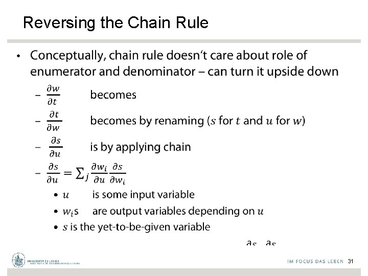
Reversing the Chain Rule • 31
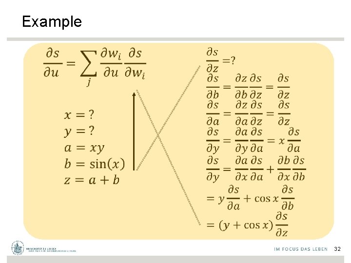
Example • • 32
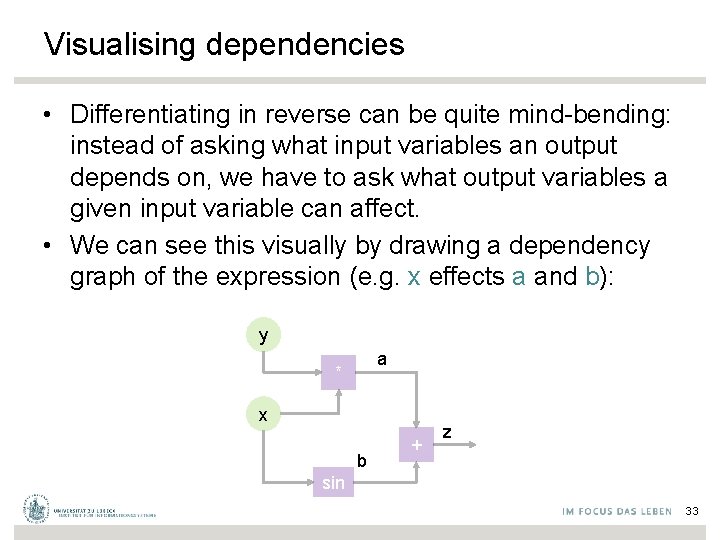
Visualising dependencies • Differentiating in reverse can be quite mind-bending: instead of asking what input variables an output depends on, we have to ask what output variables a given input variable can affect. • We can see this visually by drawing a dependency graph of the expression (e. g. x effects a and b): y a * x b + z sin 33
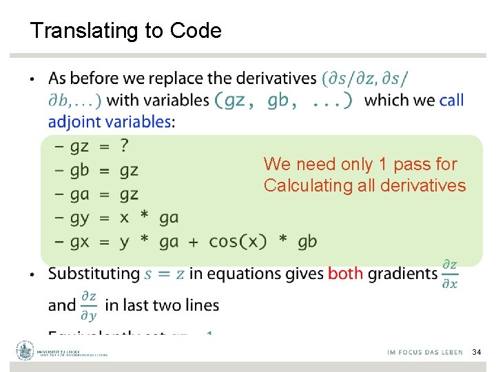
Translating to Code • We need only 1 pass for Calculating all derivatives 34
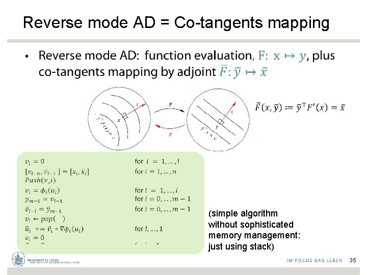
Reverse mode AD = Co-tangents mapping • (simple algorithm without sophisticated memory management: just using stack) 35
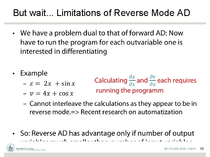
But wait. . . Limitations of Reverse Mode AD • 36
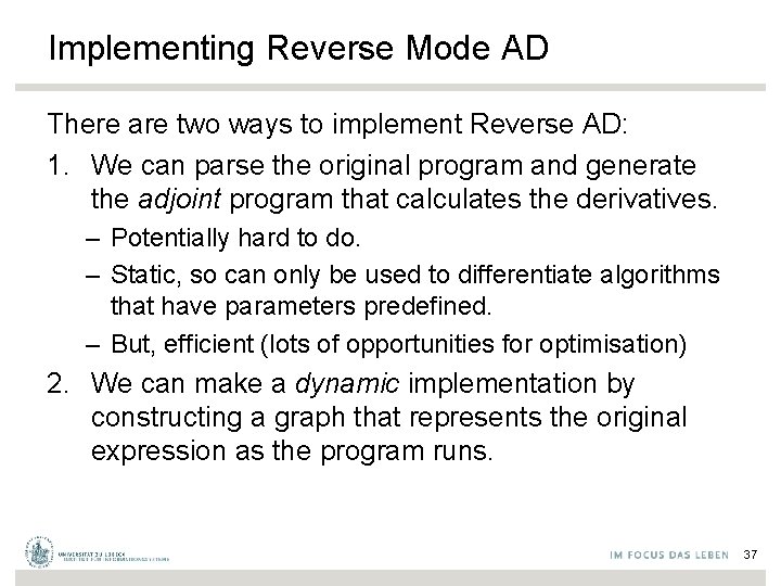
Implementing Reverse Mode AD There are two ways to implement Reverse AD: 1. We can parse the original program and generate the adjoint program that calculates the derivatives. – Potentially hard to do. – Static, so can only be used to differentiate algorithms that have parameters predefined. – But, efficient (lots of opportunities for optimisation) 2. We can make a dynamic implementation by constructing a graph that represents the original expression as the program runs. 37
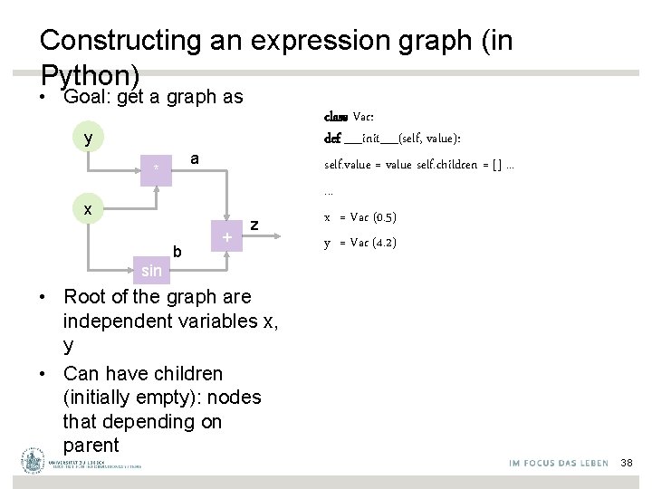
Constructing an expression graph (in Python) • Goal: get a graph as y a * x b + z class Var: def __init__(self, value): self. value = value self. children = []. . . x = Var (0. 5) y = Var (4. 2) sin • Root of the graph are independent variables x, y • Can have children (initially empty): nodes that depending on parent 38
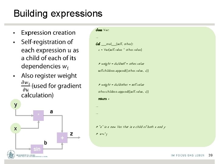
Building expressions class Var: . . . def __mul__(self, other): z = Var(self. value * other. value) • # weight = dz/dself = other. value self. children. append((other. value, z)) # weight = dz/dother = self. value other. children. append((self. value, z)) return z. . . y a * x b + z # "a" is a new Var that is a child of both x and y # a=x*y sin 39
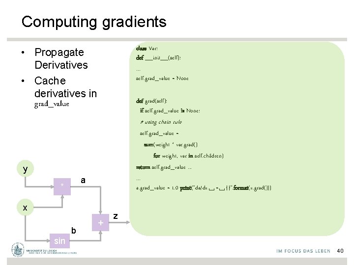
Computing gradients class Var: def __init__(self): . . . self. grad_value = None • Propagate Derivatives • Cache derivatives in grad_value def grad(self): if self. grad_value is None: # using chain rule self. grad_value = sum(weight * var. grad() for weight, var in self. children) return self. grad_value. . . a. grad_value = 1. 0 print("da/dx␣=␣{}". format(x. grad())) y a * x b + z sin 40
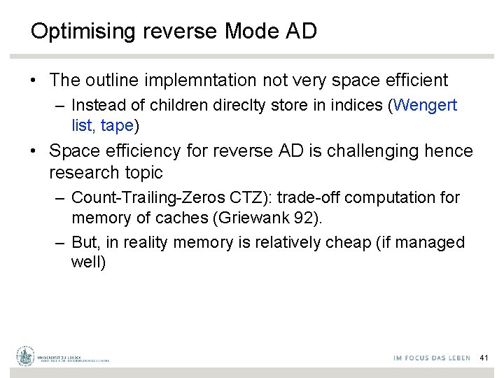
Optimising reverse Mode AD • The outline implemntation not very space efficient – Instead of children direclty store in indices (Wengert list, tape) • Space efficiency for reverse AD is challenging hence research topic – Count-Trailing-Zeros CTZ): trade-off computation for memory of caches (Griewank 92). – But, in reality memory is relatively cheap (if managed well) 41
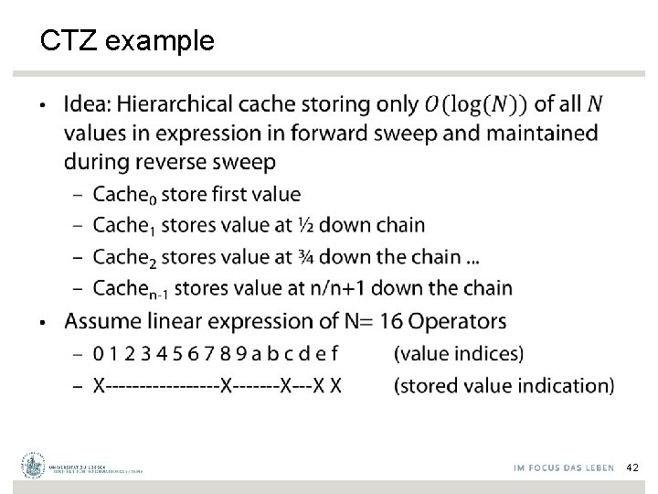
CTZ example • 42
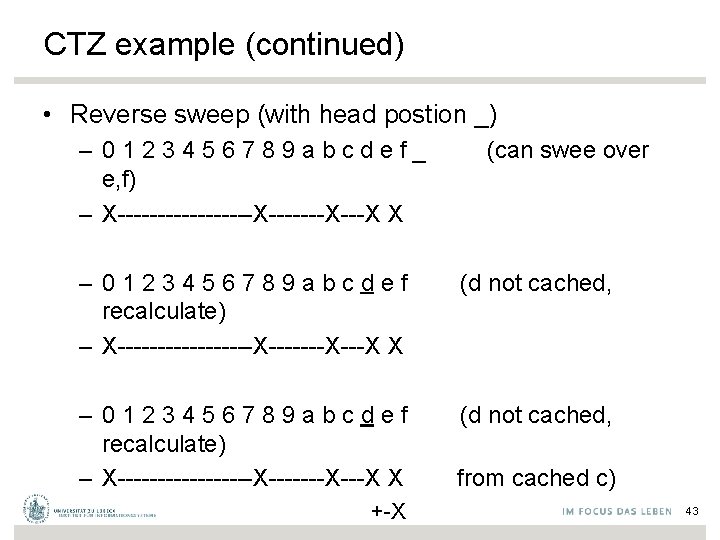
CTZ example (continued) • Reverse sweep (with head postion _) – 0 1 2 3 4 5 6 7 8 9 a b c d e f _ (can swee over e, f) – X-----------------X-------X---X X – 0 1 2 3 4 5 6 7 8 9 a b c d e f (d not cached, recalculate) – X---------X-------X X from cached c) +-X 43
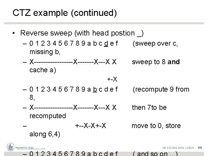
CTZ example (continued) • Reverse sweep (with head postion _) – 0 1 2 3 4 5 6 7 8 9 a b c d e f (sweep over c, missing b, – X---------X-------X X sweep to 8 and cache a) +-X – 0 1 2 3 4 5 6 7 8 9 a b c d e f (recompute 9 from 8, – X---------X-------X X then 7 to be recomputed – +--X-X+-X move to 0, store along 6, 4) 44
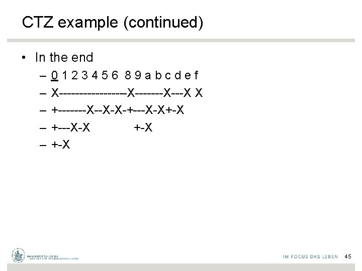
CTZ example (continued) • In the end – – – 0 1 2 3 4 5 6 8 9 a b c d e f X---------X-------X X +-------X--X-X-+---X-X+-X +---X-X +-X 45
Uhhh, a lecture with a hopefully useful APPENDIX 46
Color Convention in this Course • Formulae, when occurring inline • Newly introduced terminology and definitions • Important results (observations, theorems) as well as emphasizing some aspects • Examples are given with standard orange with possibly light orange frame • Comments and notes in nearly opaque post-it • Algorithms and program code • Reminders (in the grey fog of your memory) 47
Today‘s lecture is based on the following • Jonathon Hare: Lecture 5 of course „COMP 6248 Differentiable Programming (and some Deep Learning)“ http: //comp 6248. ecs. soton. ac. uk/ • Blog post by Rufflewind: Reverse-mode automatic differentiation: a tutorial https: //rufflewind. com/2016 - 12 - 30/reverse- mode- automatic - differentiation • A. G. Baydin, B. A. Pearlmutter, A. A. Radul, and J. M. Siskind. Automatic differentiation in machine learning: A survey. J. Mach. Learn. Res. , 18(1): 5595– 5637, Jan. 2017. • A. H. Gebremedhin and A. Walther. An introduction to algorithmic differentiation. WIREs Data Mining and Knowledge Discovery, 10(1): e 1334, 2020. 48
References • • W. K. Clifford. Preliminary sketch of bi-quaternions. Proceedings of the London Mathematical Society, pages 381 — 395, 1873. A. Griewank. Achieving logarithmic growth of temporal and spatial complexity in reverse automatic differentiation. Optimization Methods and Software, 1(1): 35– 54, 1992. 49
- Slides: 49