Privacy Preserving Data Mining Challenges Opportunities Ramakrishnan Srikant

Privacy Preserving Data Mining: Challenges & Opportunities Ramakrishnan Srikant

Growing Privacy Concerns • Popular Press: – Economist: The End of Privacy (May 99) – Time: The Death of Privacy (Aug 97) • Govt. directives/commissions: – European directive on privacy protection (Oct 98) – Canadian Personal Information Protection Act (Jan 2001) • Special issue on internet privacy, CACM, Feb 99 • S. Garfinkel, "Database Nation: The Death of Privacy in 21 st Century", O' Reilly, Jan 2000

Privacy Concerns (2) • Surveys of web users – 17% privacy fundamentalists, 56% pragmatic majority, 27% marginally concerned (Understanding net users' attitude about online privacy, April 99) – 82% said having privacy policy would matter (Freebies & Privacy: What net users think, July 99)

Technical Question • Fear: – "Join" (record overlay) was the original sin. – Data mining: new, powerful adversary? • The primary task in data mining: development of models about aggregated data. • Can we develop accurate models without access to precise information in individual data records?

Talk Overview • Motivation • Randomization Approach – R. Agrawal and R. Srikant, “Privacy Preserving Data Mining”, SIGMOD 2000. – Application: Web Demographics • Cryptographic Approach – Application: Inter-Enterprise Data Mining • Challenges – Application: Privacy-Sensitive Security Profiling

Web Demographics • Volvo S 40 website targets people in 20 s – Are visitors in their 20 s or 40 s? – Which demographic groups like/dislike the website?

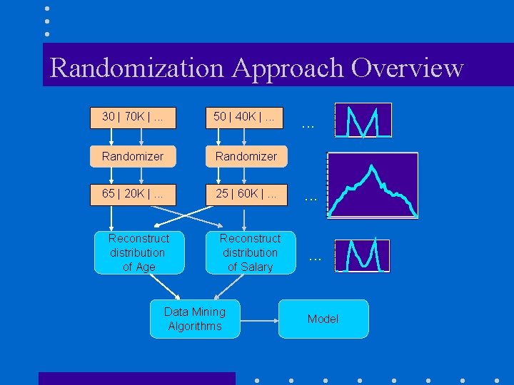
Randomization Approach Overview 30 | 70 K |. . . 50 | 40 K |. . . Randomizer 65 | 20 K |. . . 25 | 60 K |. . . Reconstruct distribution of Age Reconstruct distribution of Salary Data Mining Algorithms . . Model

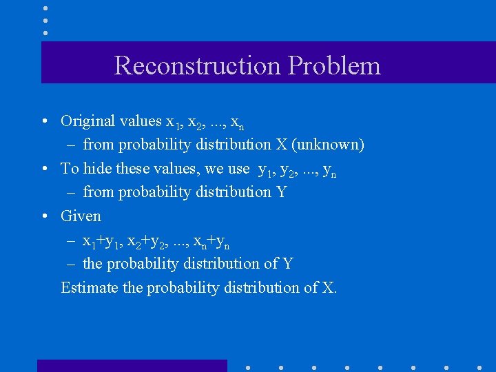
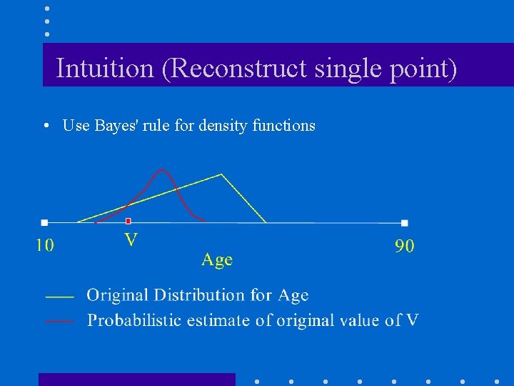
Reconstruction Problem • Original values x 1, x 2, . . . , xn – from probability distribution X (unknown) • To hide these values, we use y 1, y 2, . . . , yn – from probability distribution Y • Given – x 1+y 1, x 2+y 2, . . . , xn+yn – the probability distribution of Y Estimate the probability distribution of X.

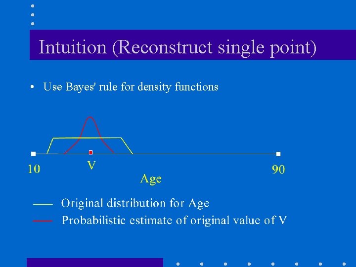
Intuition (Reconstruct single point) • Use Bayes' rule for density functions

Intuition (Reconstruct single point) • Use Bayes' rule for density functions

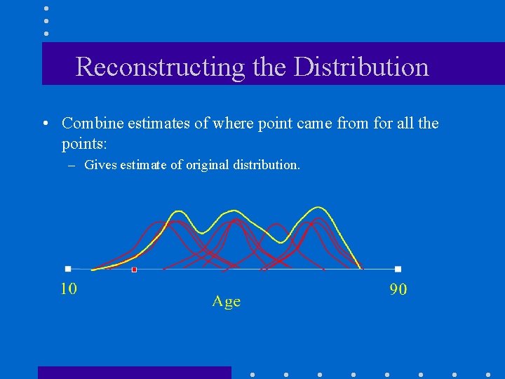
Reconstructing the Distribution • Combine estimates of where point came from for all the points: – Gives estimate of original distribution.

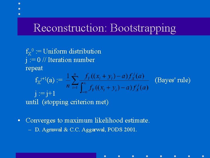
Reconstruction: Bootstrapping f. X 0 : = Uniform distribution j : = 0 // Iteration number repeat f. Xj+1(a) : = j+1 until (stopping criterion met) • Converges to maximum likelihood estimate. – D. Agrawal & C. C. Aggarwal, PODS 2001. (Bayes' rule)

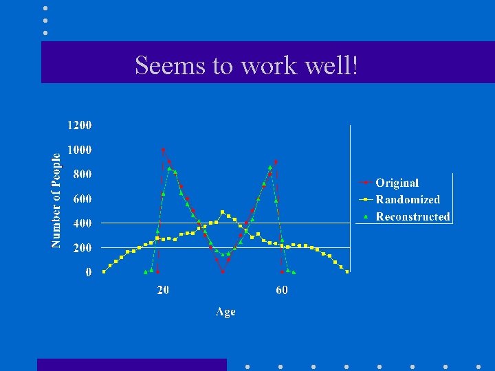
Seems to work well!

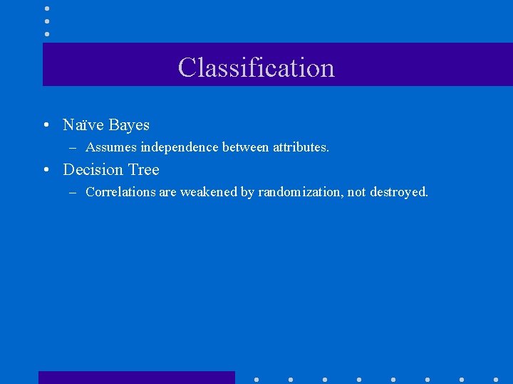
Classification • Naïve Bayes – Assumes independence between attributes. • Decision Tree – Correlations are weakened by randomization, not destroyed.

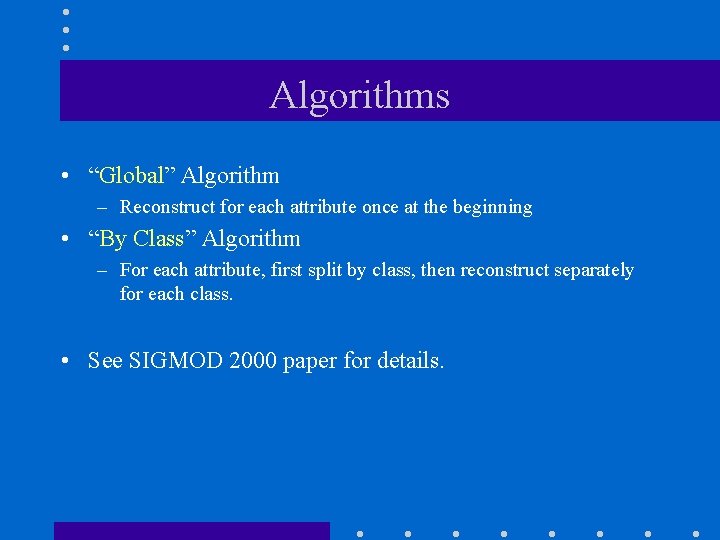
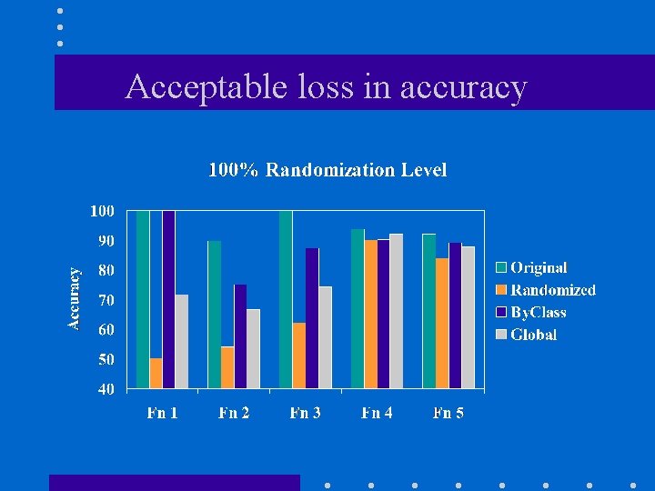
Algorithms • “Global” Algorithm – Reconstruct for each attribute once at the beginning • “By Class” Algorithm – For each attribute, first split by class, then reconstruct separately for each class. • See SIGMOD 2000 paper for details.

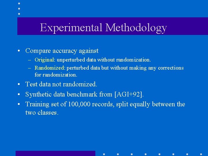
Experimental Methodology • Compare accuracy against – Original: unperturbed data without randomization. – Randomized: perturbed data but without making any corrections for randomization. • Test data not randomized. • Synthetic data benchmark from [AGI+92]. • Training set of 100, 000 records, split equally between the two classes.

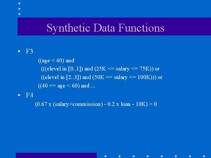
Synthetic Data Functions • F 3 ((age < 40) and (((elevel in [0. . 1]) and (25 K <= salary <= 75 K)) or ((elevel in [2. . 3]) and (50 K <= salary <= 100 K))) or ((40 <= age < 60) and. . . • F 4 (0. 67 x (salary+commission) - 0. 2 x loan - 10 K) > 0

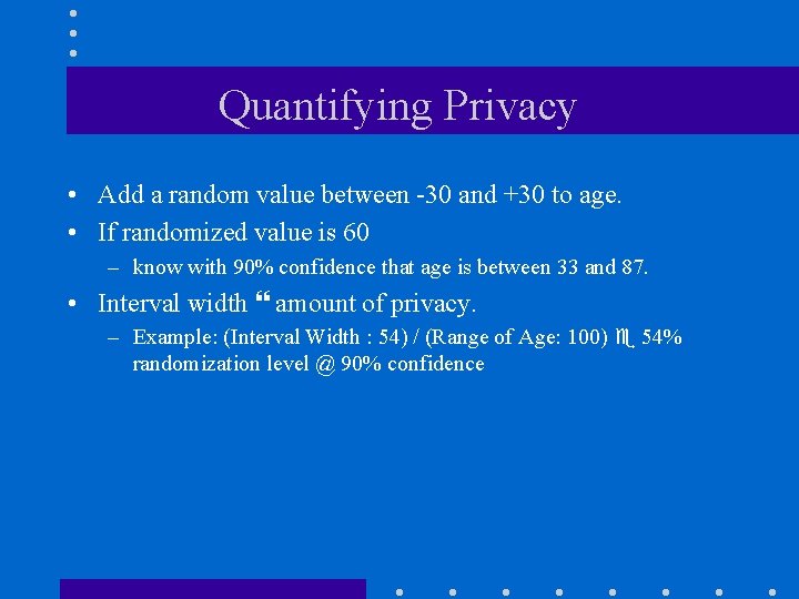
Quantifying Privacy • Add a random value between -30 and +30 to age. • If randomized value is 60 – know with 90% confidence that age is between 33 and 87. • Interval width amount of privacy. – Example: (Interval Width : 54) / (Range of Age: 100) 54% randomization level @ 90% confidence

Acceptable loss in accuracy

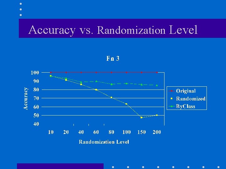
Accuracy vs. Randomization Level

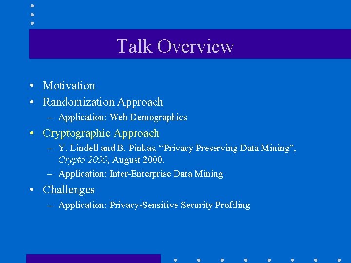
Talk Overview • Motivation • Randomization Approach – Application: Web Demographics • Cryptographic Approach – Y. Lindell and B. Pinkas, “Privacy Preserving Data Mining”, Crypto 2000, August 2000. – Application: Inter-Enterprise Data Mining • Challenges – Application: Privacy-Sensitive Security Profiling

Inter-Enterprise Data Mining • Problem: Two parties owning confidential databases wish to build a decision-tree classifier on the union of their databases, without revealing any unnecessary information. • Horizontally partitioned. – Records (users) split across companies. – Example: Credit card fraud detection model. • Vertically partitioned. – Attributes split across companies. – Example: Associations across websites.

Cryptographic Adversaries • Malicious adversary: can alter its input, e. g. , define input to be the empty database. • Semi-honest (or passive) adversary: Correctly follows the protocol specification, yet attempts to learn additional information by analyzing the messages.

Yao's two-party protocol • • Party 1 with input x Party 2 with input y Wish to compute f(x, y) without revealing x, y. Yao, “How to generate and exchange secrets”, FOCS 1986.

Private Distributed ID 3 • Key problem: find attribute with highest information gain. • We can then split on this attribute and recurse. – Assumption: Numeric values are discretized, with n-way split.

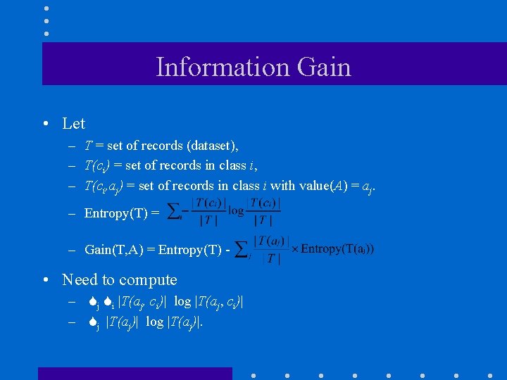
Information Gain • Let – T = set of records (dataset), – T(ci) = set of records in class i, – T(ci, aj) = set of records in class i with value(A) = aj. – Entropy(T) = – Gain(T, A) = Entropy(T) - • Need to compute – Sj Si |T(aj, ci)| log |T(aj, ci)| – Sj |T(aj)| log |T(aj)|.

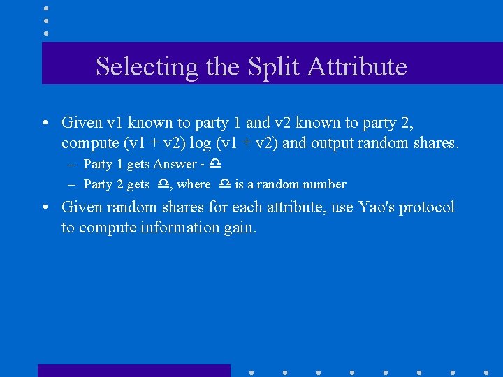
Selecting the Split Attribute • Given v 1 known to party 1 and v 2 known to party 2, compute (v 1 + v 2) log (v 1 + v 2) and output random shares. – Party 1 gets Answer - d – Party 2 gets d, where d is a random number • Given random shares for each attribute, use Yao's protocol to compute information gain.

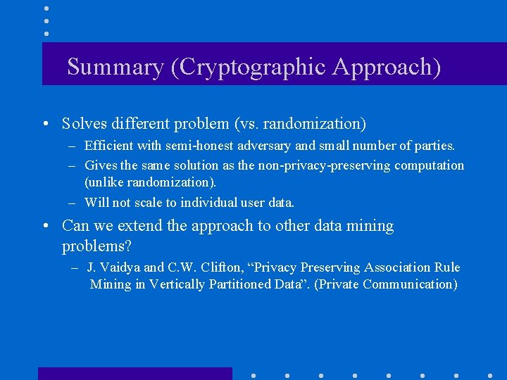
Summary (Cryptographic Approach) • Solves different problem (vs. randomization) – Efficient with semi-honest adversary and small number of parties. – Gives the same solution as the non-privacy-preserving computation (unlike randomization). – Will not scale to individual user data. • Can we extend the approach to other data mining problems? – J. Vaidya and C. W. Clifton, “Privacy Preserving Association Rule Mining in Vertically Partitioned Data”. (Private Communication)

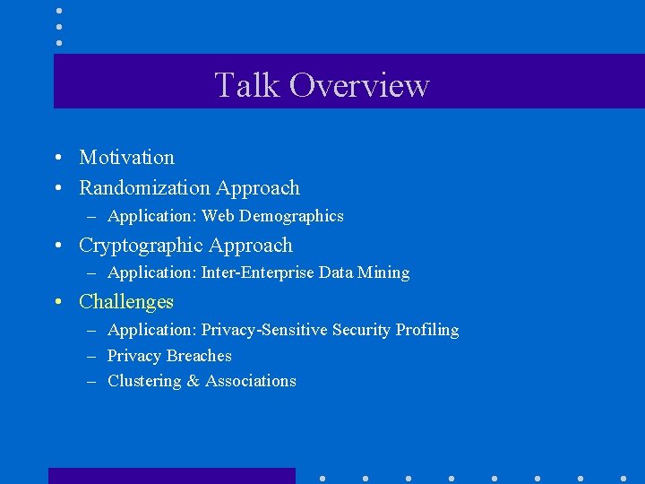
Talk Overview • Motivation • Randomization Approach – Application: Web Demographics • Cryptographic Approach – Application: Inter-Enterprise Data Mining • Challenges – Application: Privacy-Sensitive Security Profiling – Privacy Breaches – Clustering & Associations

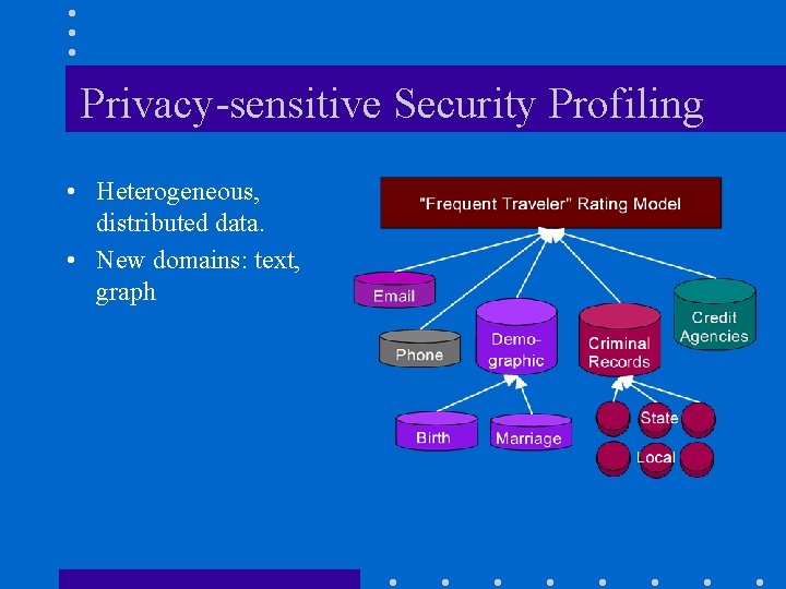
Privacy-sensitive Security Profiling • Heterogeneous, distributed data. • New domains: text, graph

Potential Privacy Breaches • Distribution is a spike. – Example: Everyone is of age 40. • Some randomized values are only possible from a given range. – Example: Add U[-50, +50] to age and get 125 True age is 75. – Not an issue with Gaussian.

Potential Privacy Breaches (2) • Most randomized values in a given interval come from a given interval. – Example: 60% of the people whose randomized value is in [120, 130] have their true age in [70, 80]. – Implication: Higher levels of randomization will be required. • Correlations can make previous effect worse. – Example: 80% of the people whose randomized value of age is in [120, 130] and whose randomized value of income is [. . . ] have their true age in [70, 80]. • Challenge: How do you limit privacy breaches?

Clustering • Classification: By. Class partitioned the data by class & then reconstructed attributes. – Assumption: Attributes independent given class attribute. • Clustering: Don’t know the class label. – Assumption: Attributes independent. • Global (latter assumption) does much worse than By. Class. • Can we reconstruct a set of attributes together? – Amount of data needed increases exponentially with number of attributes.

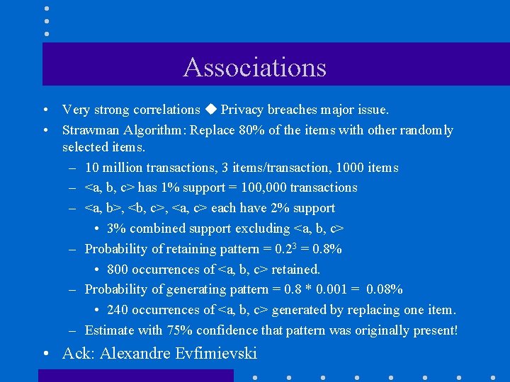
Associations • Very strong correlations Privacy breaches major issue. • Strawman Algorithm: Replace 80% of the items with other randomly selected items. – 10 million transactions, 3 items/transaction, 1000 items – <a, b, c> has 1% support = 100, 000 transactions – <a, b>, <b, c>, <a, c> each have 2% support • 3% combined support excluding <a, b, c> – Probability of retaining pattern = 0. 23 = 0. 8% • 800 occurrences of <a, b, c> retained. – Probability of generating pattern = 0. 8 * 0. 001 = 0. 08% • 240 occurrences of <a, b, c> generated by replacing one item. – Estimate with 75% confidence that pattern was originally present! • Ack: Alexandre Evfimievski

Summary • Have your cake and mine it too! – Preserve privacy at the individual level, but still build accurate models. • Challenges – Privacy Breaches, Security Applications, Clustering & Associations • Opportunities – Web Demographics, Inter-Enterprise Data Mining, Security Applications www. almaden. ibm. com/cs/people/srikant/talks. html

Backup

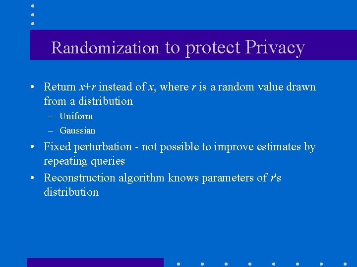
Randomization to protect Privacy • Return x+r instead of x, where r is a random value drawn from a distribution – Uniform – Gaussian • Fixed perturbation - not possible to improve estimates by repeating queries • Reconstruction algorithm knows parameters of r's distribution

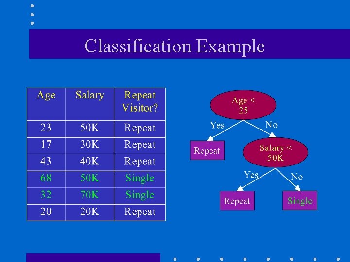
Classification Example

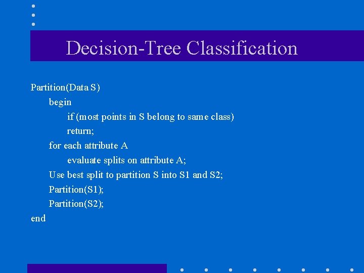
Decision-Tree Classification Partition(Data S) begin if (most points in S belong to same class) return; for each attribute A evaluate splits on attribute A; Use best split to partition S into S 1 and S 2; Partition(S 1); Partition(S 2); end

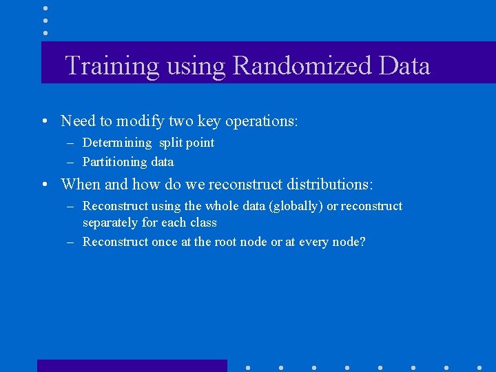
Training using Randomized Data • Need to modify two key operations: – Determining split point – Partitioning data • When and how do we reconstruct distributions: – Reconstruct using the whole data (globally) or reconstruct separately for each class – Reconstruct once at the root node or at every node?

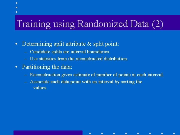
Training using Randomized Data (2) • Determining split attribute & split point: – Candidate splits are interval boundaries. – Use statistics from the reconstructed distribution. • Partitioning the data: – Reconstruction gives estimate of number of points in each interval. – Associate each data point with an interval by sorting the values.

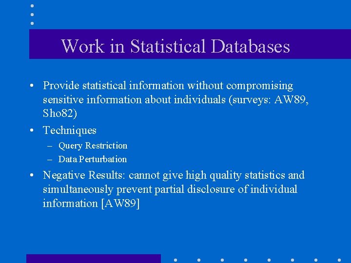
Work in Statistical Databases • Provide statistical information without compromising sensitive information about individuals (surveys: AW 89, Sho 82) • Techniques – Query Restriction – Data Perturbation • Negative Results: cannot give high quality statistics and simultaneously prevent partial disclosure of individual information [AW 89]

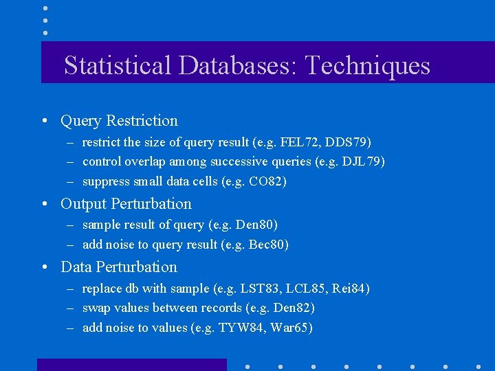
Statistical Databases: Techniques • Query Restriction – restrict the size of query result (e. g. FEL 72, DDS 79) – control overlap among successive queries (e. g. DJL 79) – suppress small data cells (e. g. CO 82) • Output Perturbation – sample result of query (e. g. Den 80) – add noise to query result (e. g. Bec 80) • Data Perturbation – replace db with sample (e. g. LST 83, LCL 85, Rei 84) – swap values between records (e. g. Den 82) – add noise to values (e. g. TYW 84, War 65)

Statistical Databases: Comparison • We do not assume original data is aggregated into a single database. • Concept of reconstructing original distribution. – Adding noise to data values problematic without such reconstruction.