Principles of the MRI Signal Contrast Mechanisms MR

Principles of the MRI Signal Contrast Mechanisms MR Image Formation John Van. Meter, Ph. D. Center for Functional and Molecular Imaging Georgetown University Medical Center

Outline • Physics behind MRI • Basis of the MRI signal • Tissue Contrast • Examples • Spatial Localization

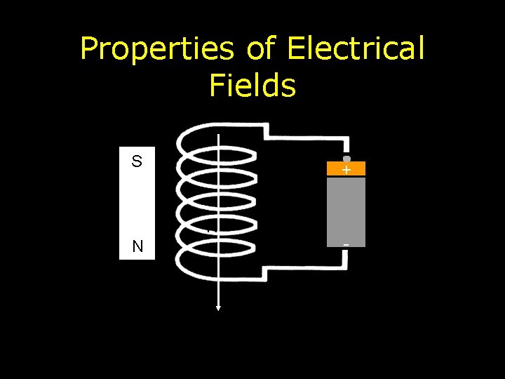
Properties of Electrical Fields S S + N N -

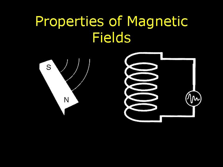
Properties of Magnetic Fields S N

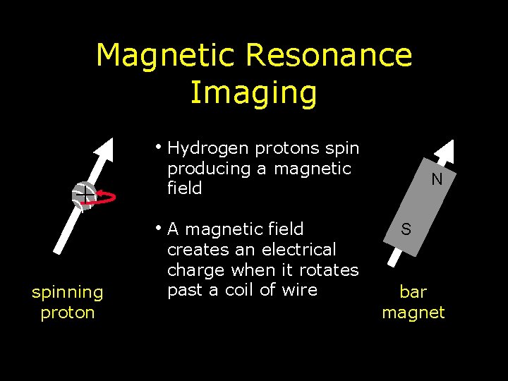
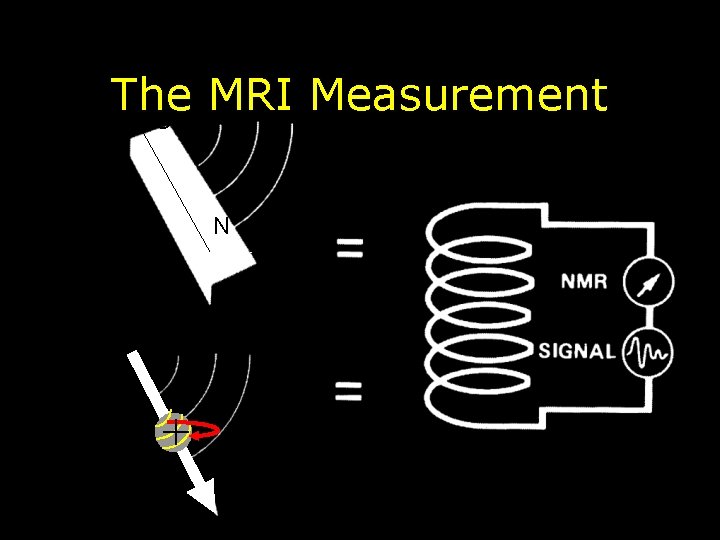
Magnetic Resonance Imaging • Hydrogen protons spin + producing a magnetic field • A magnetic field spinning proton creates an electrical charge when it rotates past a coil of wire N S bar magnet

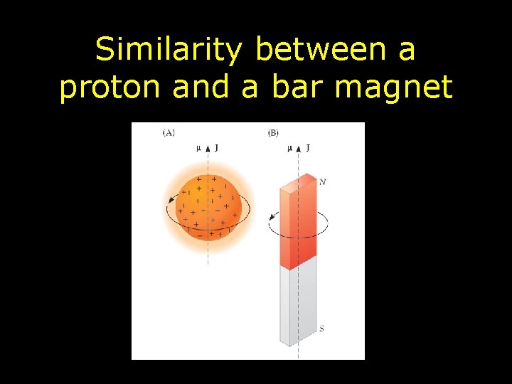
Similarity between a proton and a bar magnet

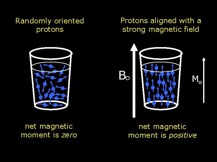
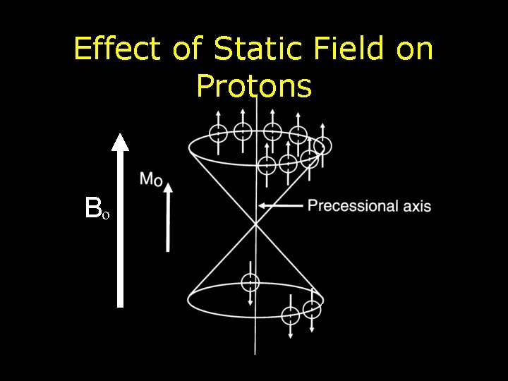
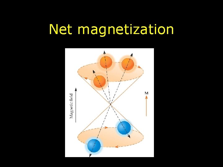
Randomly oriented protons Protons aligned with a strong magnetic field Bo net magnetic moment is zero Mo net magnetic moment is positive

The MRI Measurement S N +

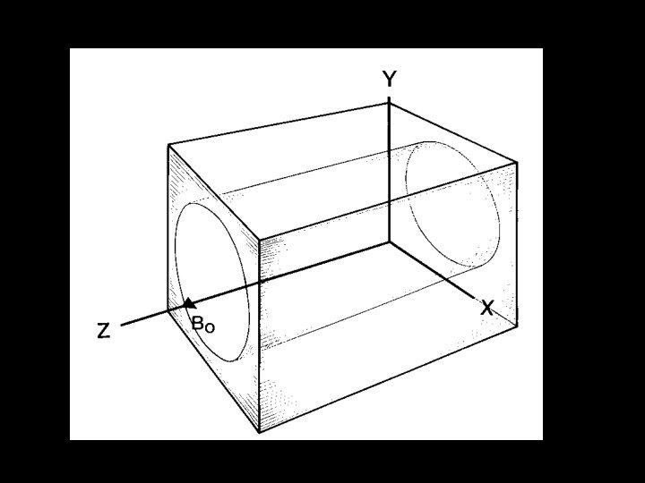
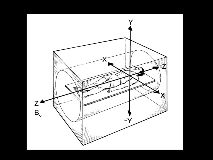
Effect of Static Field on Protons Bo

Net magnetization

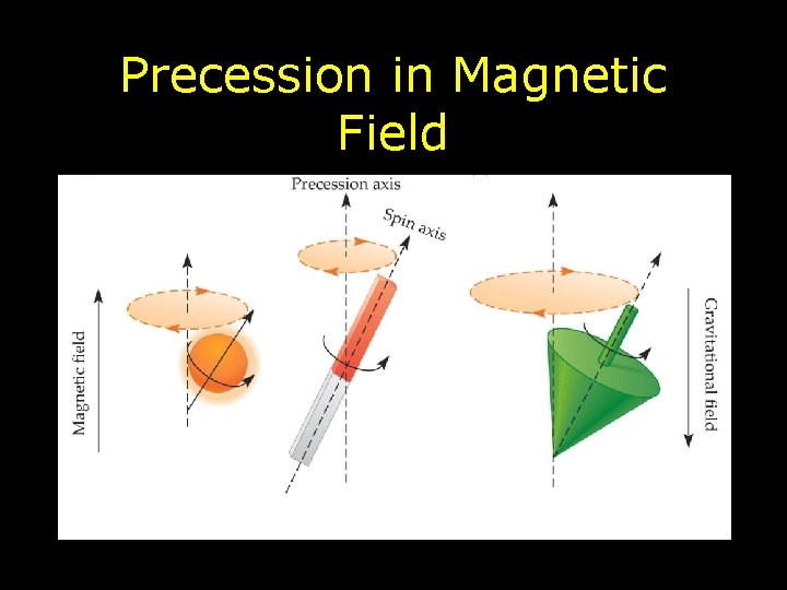
Precession in Magnetic Field

Bo

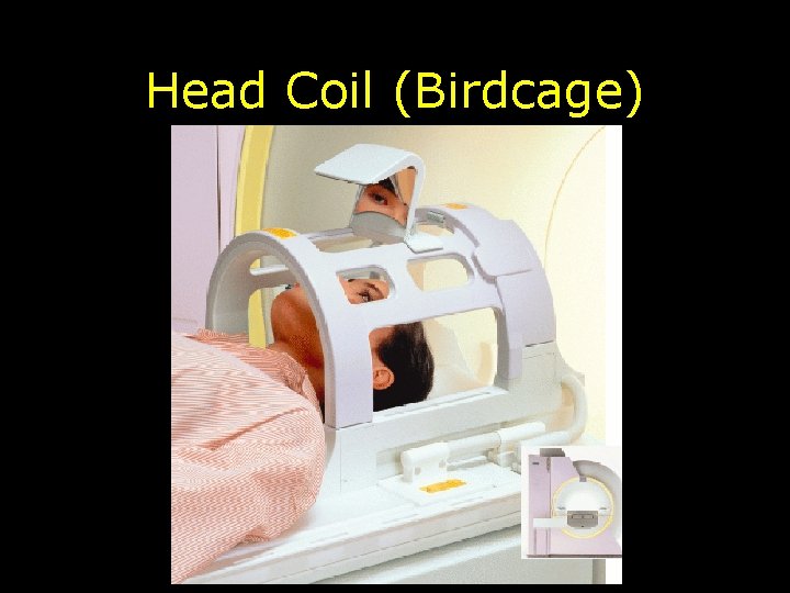
Head Coil (Birdcage)

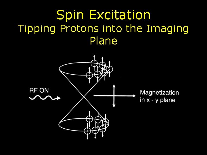
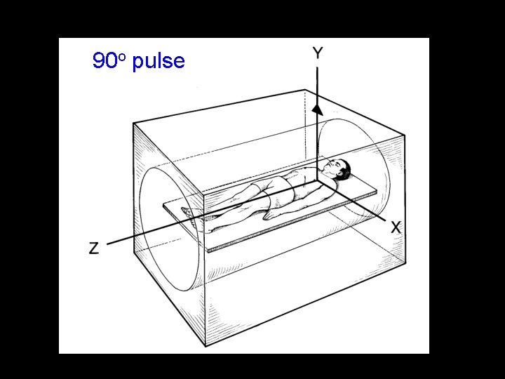
Spin Excitation Tipping Protons into the Imaging Plane

90 o pulse

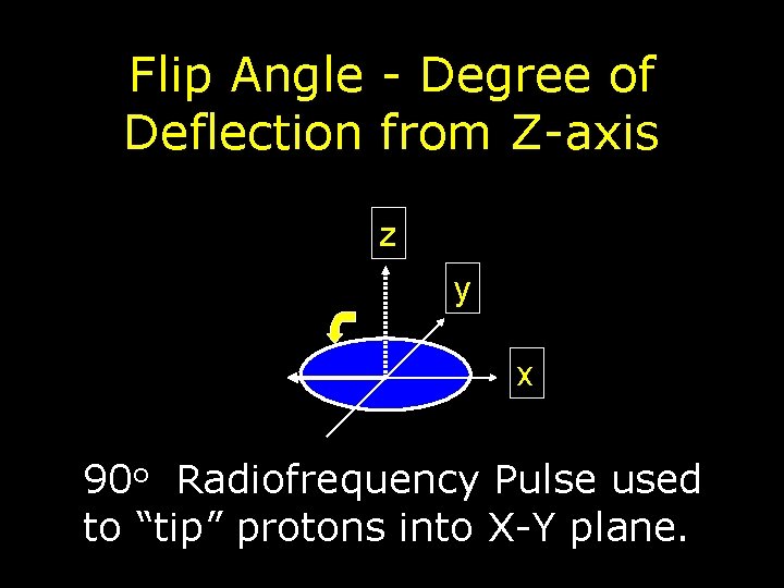
Flip Angle - Degree of Deflection from Z-axis z y x 90 o Radiofrequency Pulse used to “tip” protons into X-Y plane.

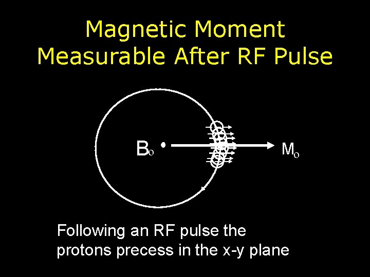
Magnetic Moment Measurable After RF Pulse Bo Mo Following an RF pulse the protons precess in the x-y plane

The MRI Measurement (Up to this point) • In the presence of the static magnetic field – Protons align with the field – Protons precess about the magnetic • Briefly turn on RF pulse – Provides energy to tip the protons at least partially into the imaging plane • What happens to the protons next?

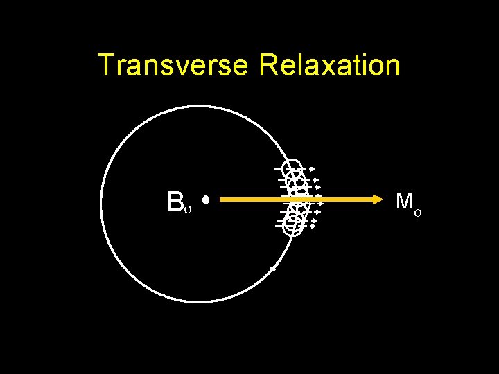
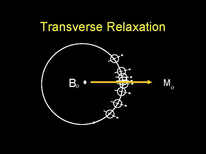
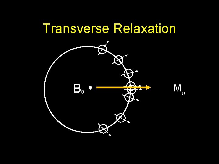
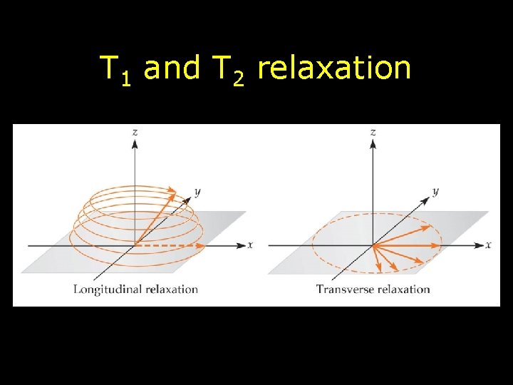
Types of Relaxation • Longitudinal – precessing protons are pulled back into alignment with main magnetic field of the scanner (Bo) reducing size of the magnetic moment vector in the x-y plane • Transverse – precessing protons become out of phase leading to a drop in the net magnetic moment vector (Mo) • Transverse relaxation occurs much faster than Longitudinal relaxation • Tissue contrast is determined by differences in these two types of relaxation

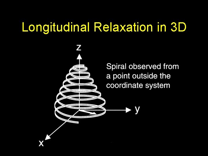
Longitudinal Relaxation in 3 D

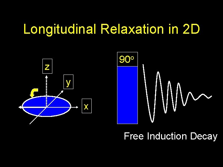
Longitudinal Relaxation in 2 D 90 o z y x Free Induction Decay

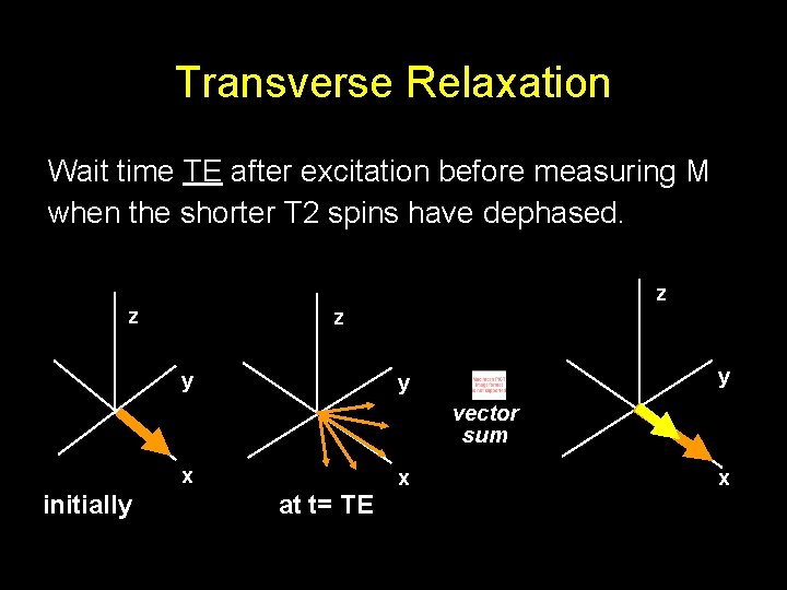
Transverse Relaxation Wait time TE after excitation before measuring M when the shorter T 2 spins have dephased. z z z y y y vector sum x initially at t= TE x x

Transverse Relaxation Bo Mo

Transverse Relaxation Bo Mo

Transverse Relaxation Bo Mo

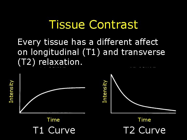
T 1 and T 2 relaxation

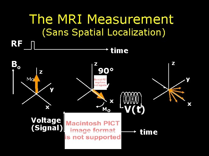
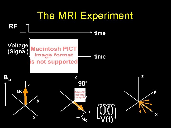
The MRI Measurement (Sans Spatial Localization) RF time Bo z z Mo y x Voltage (Signal) z 90° y Mo x Mo V(t) time ty x

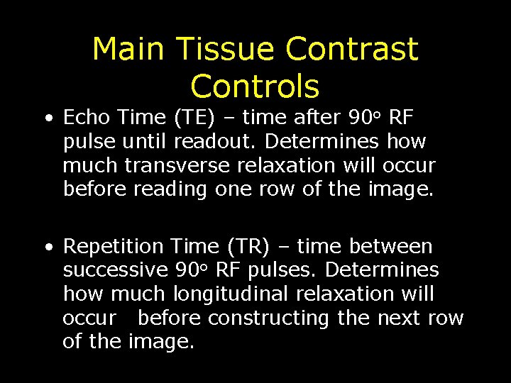
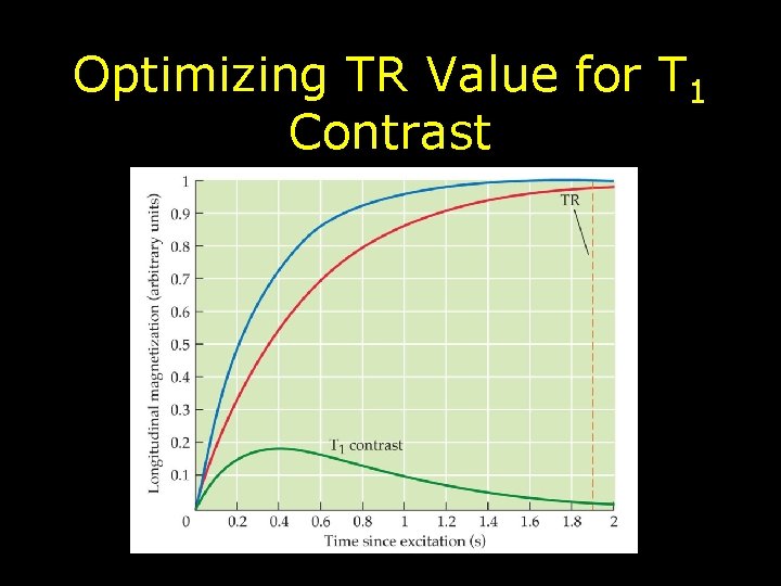
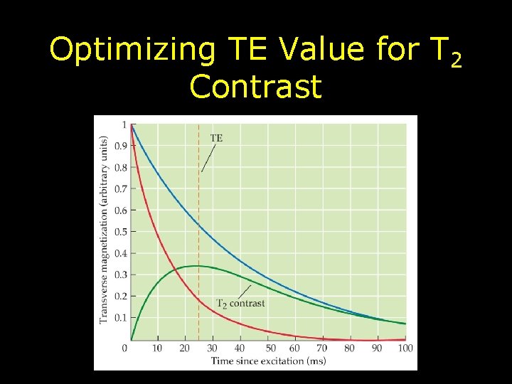
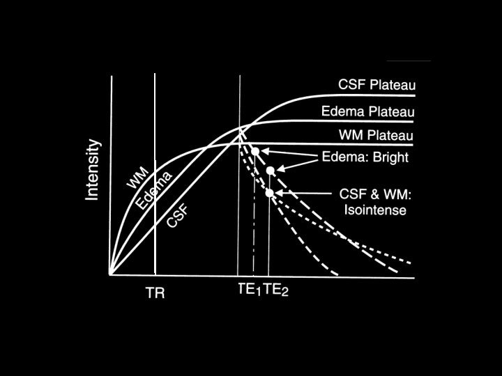
Main Tissue Contrast Controls • Echo Time (TE) – time after 90 o RF pulse until readout. Determines how much transverse relaxation will occur before reading one row of the image. • Repetition Time (TR) – time between successive 90 o RF pulses. Determines how much longitudinal relaxation will occur before constructing the next row of the image.

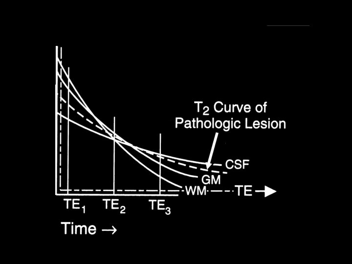
Tissue Contrast Intensity Every tissue has a different affect on longitudinal (T 1) and transverse (T 2) relaxation. Time T 1 Curve T 2 Curve

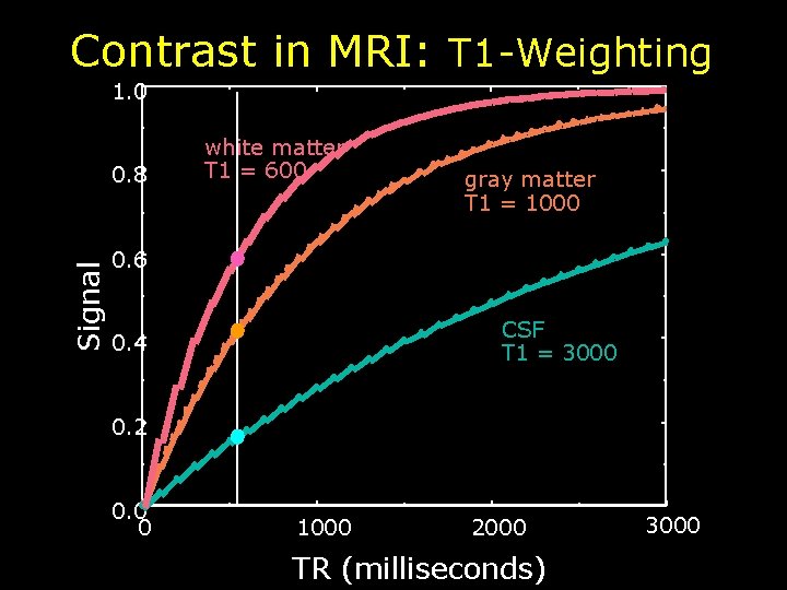
Contrast in MRI: T 1 -Weighting 1. 0 Signal 0. 8 white matter T 1 = 600 gray matter T 1 = 1000 0. 6 CSF T 1 = 3000 0. 4 0. 2 0. 0 0 1000 2000 TR (milliseconds) 3000

Optimizing TR Value for T 1 Contrast

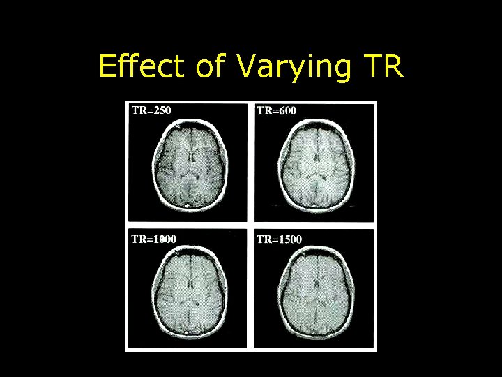
Effect of Varying TR

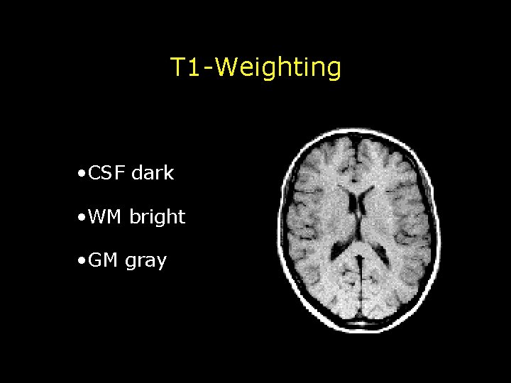
T 1 -Weighting • CSF dark • WM bright • GM gray

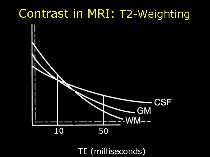
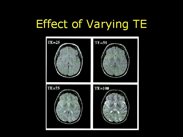
Contrast in MRI: T 2 -Weighting 10 50 TE (milliseconds)

Optimizing TE Value for T 2 Contrast

Effect of Varying TE

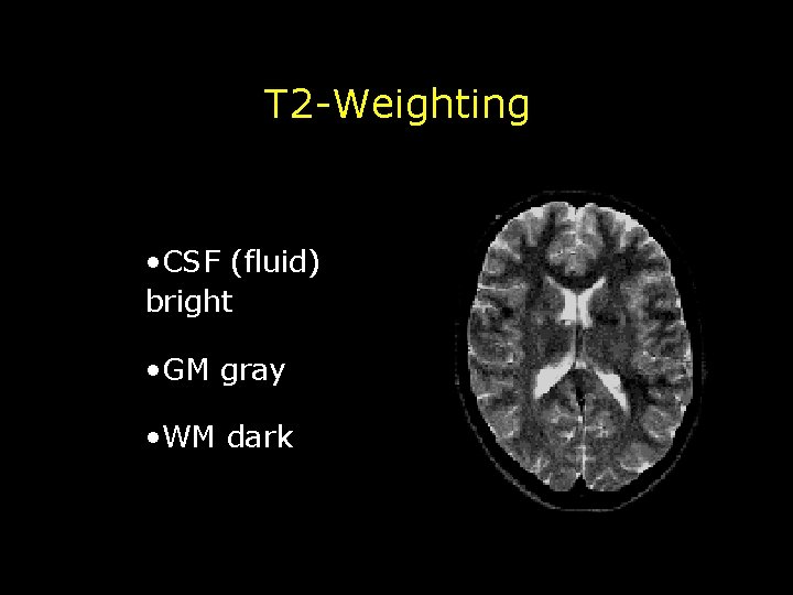
T 2 -Weighting • CSF (fluid) bright • GM gray • WM dark

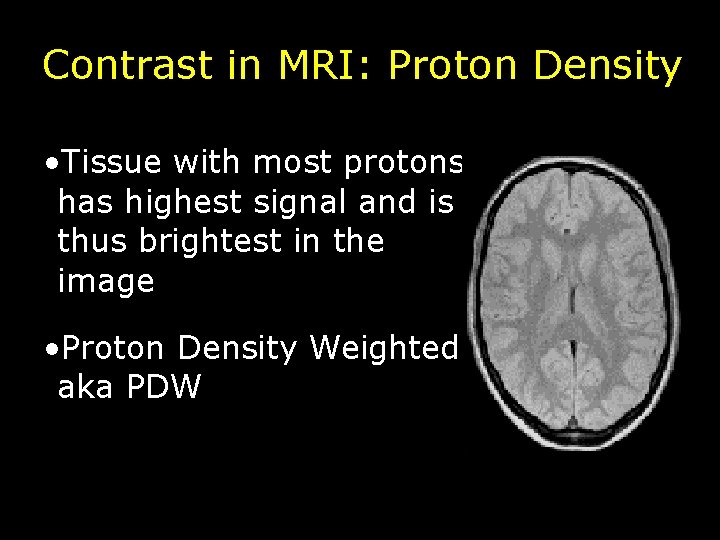
Contrast in MRI: Proton Density • Tissue with most protons has highest signal and is thus brightest in the image • Proton Density Weighted aka PDW

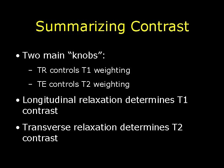
Summarizing Contrast • Two main “knobs”: – TR controls T 1 weighting – TE controls T 2 weighting • Longitudinal relaxation determines T 1 contrast • Transverse relaxation determines T 2 contrast

But Wait • How do you set TE to generate a T 1 weighted image? • How do you set TR to generate a T 2 weighted image? • How do you set TR & TE to generate a proton density weighted image?

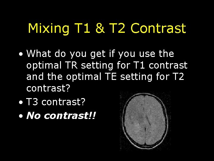
Mixing T 1 & T 2 Contrast • What do you get if you use the optimal TR setting for T 1 contrast and the optimal TE setting for T 2 contrast? • T 3 contrast? • No contrast!!

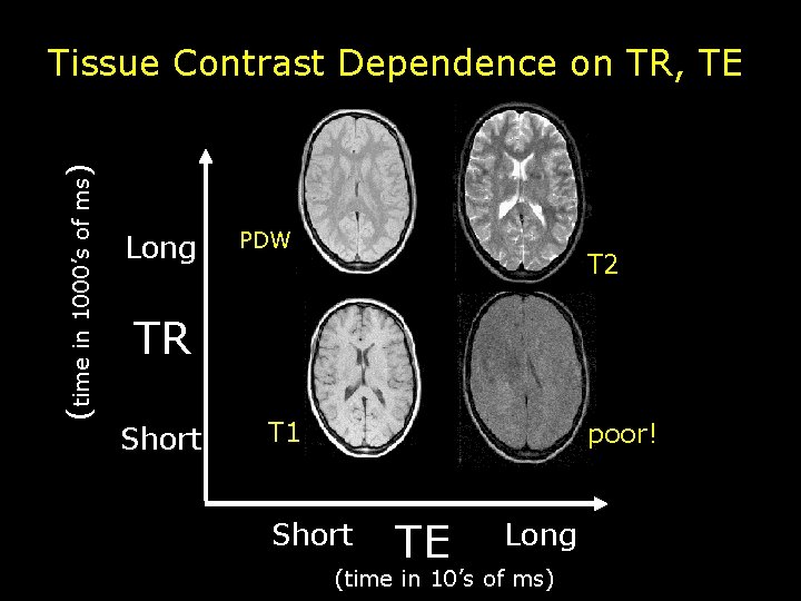
(time in 1000’s of ms) Tissue Contrast Dependence on TR, TE Long PDW T 2 TR Short T 1 poor! Short TE Long (time in 10’s of ms)

Damadian’s Discovery • Differential longitudinal relaxation between healthy and tumorous tissue in the rat • Walker sarcoma had longer T 1 relaxation time than healthy brain • Novikoff Hepatoma had shorter T 2 relaxation time than healthy liver

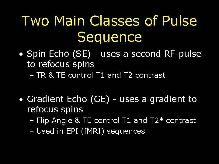
Two Main Classes of Pulse Sequence • Spin Echo (SE) - uses a second RF-pulse to refocus spins – TR & TE control T 1 and T 2 contrast • Gradient Echo (GE) - uses a gradient to refocus spins – Flip Angle & TE control T 1 and T 2* contrast – Used in EPI (f. MRI) sequences

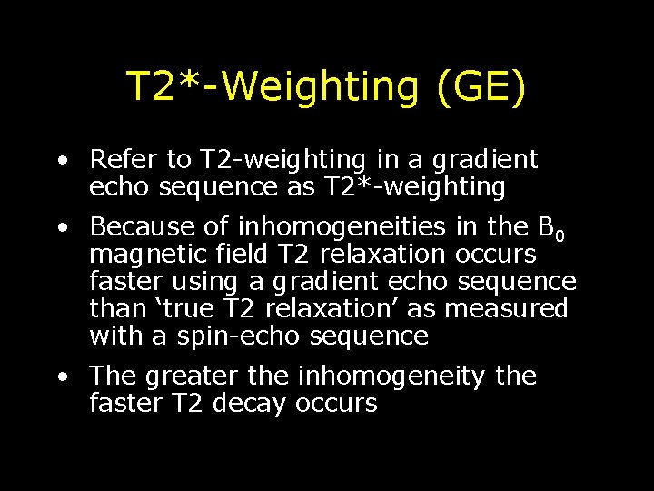
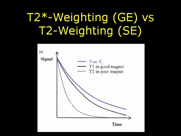
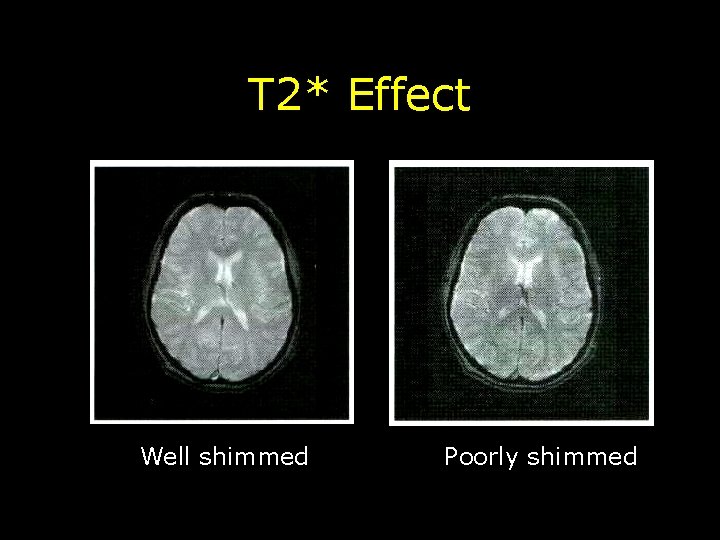
T 2*-Weighting (GE) • Refer to T 2 -weighting in a gradient echo sequence as T 2*-weighting • Because of inhomogeneities in the B 0 magnetic field T 2 relaxation occurs faster using a gradient echo sequence than ‘true T 2 relaxation’ as measured with a spin-echo sequence • The greater the inhomogeneity the faster T 2 decay occurs

T 2*-Weighting (GE) vs T 2 -Weighting (SE)

T 2* Effect Well shimmed Poorly shimmed

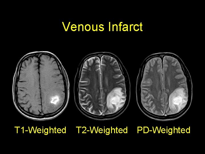
Venous Infarct T 1 -Weighted T 2 -Weighted PD-Weighted

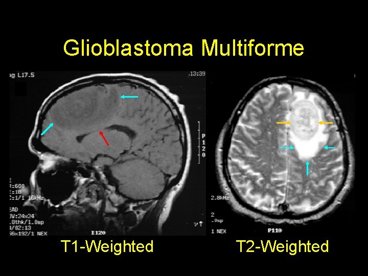
Glioblastoma Multiforme T 1 -Weighted T 2 -Weighted

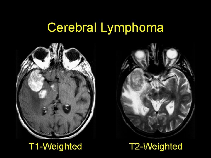
Cerebral Lymphoma T 1 -Weighted T 2 -Weighted

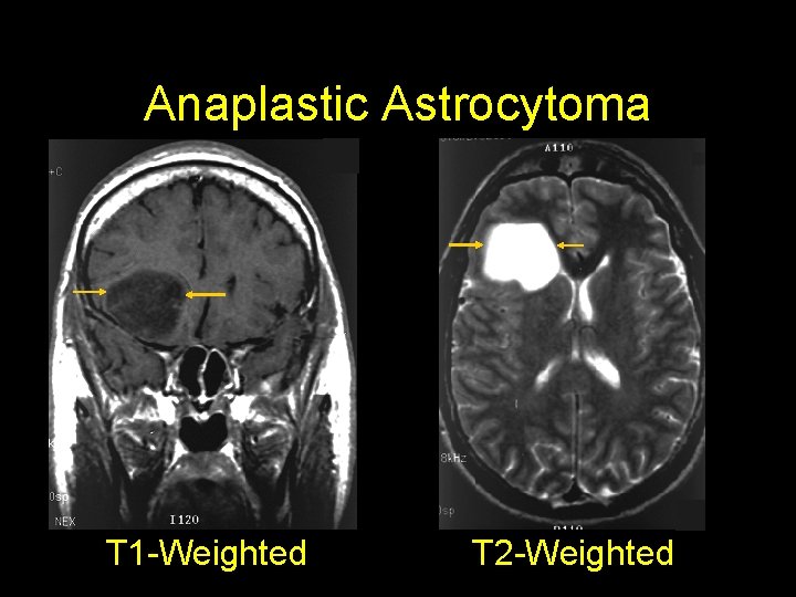
Anaplastic Astrocytoma T 1 -Weighted T 2 -Weighted

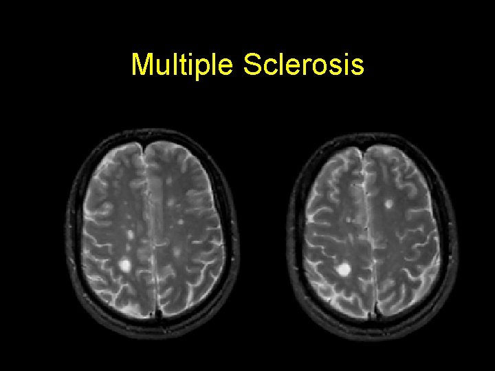
Multiple Sclerosis

The MRI Experiment RF time Voltage (Signal) time t Mo Bo z z 90° z y Mo y y x x Mo V(t) x

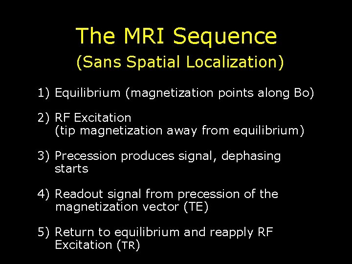
The MRI Sequence (Sans Spatial Localization) 1) Equilibrium (magnetization points along Bo) 2) RF Excitation (tip magnetization away from equilibrium) 3) Precession produces signal, dephasing starts 4) Readout signal from precession of the magnetization vector (TE) 5) Return to equilibrium and reapply RF Excitation (TR)

Spatial Localization • Gradients, linear change in magnetic field, will provide additional information needed to localize signal • Makes imaging possible/practical – Remember the Indomitable? – Couldn’t spatially localize MRI signal instead moved subject to get each voxel • Nobel prize awarded for this idea!

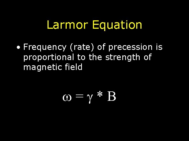
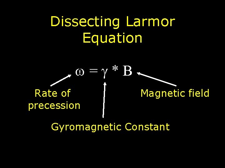
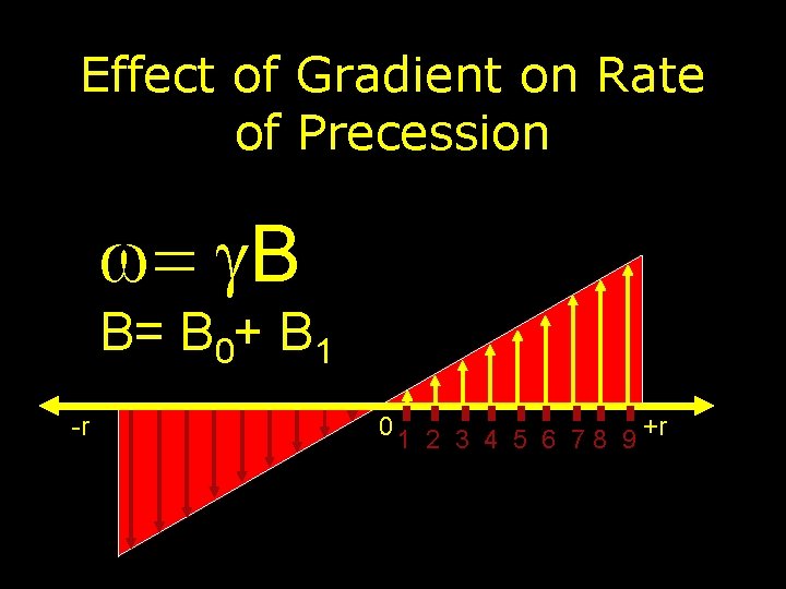
Larmor Equation • Frequency (rate) of precession is proportional to the strength of magnetic field = *B

Dissecting Larmor Equation = * B Rate of precession Magnetic field Gyromagnetic Constant

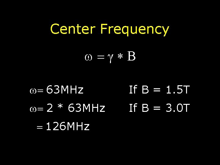
Center Frequency • Center frequency is the frequency (i. e. rate) at which protons spin (precess) with just the static magnetic field • If the center frequency of a 1. 5 T scanner is 63 MHz what it the center frequency of our 3. 0 T scanner?

Center Frequency = * B = 63 MHz If B = 1. 5 T = 2 * 63 MHz If B = 3. 0 T = 126 MHz

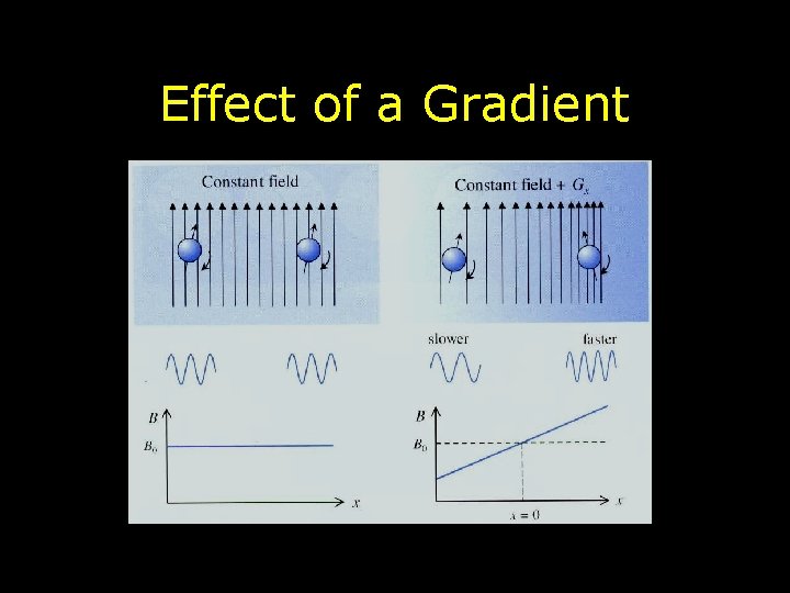
Gradients • A gradient is simply a deliberate change in the magnetic field • Gradients are used in MRI to linearly modify the magnetic field from one point in space to another • Gradients are applied along an axis (i. e. Gx along the x-axis, Gy along the y-axis, Gz along the z-axis) • What happens to the frequency at which the precess when we turn on a gradient?

Effect of Gradient on Rate of Precession = B B= B 0+ B 1 -r 0 1 2 3 4 5 6 7 8 9 +r

Effect of a Gradient

From Proton Signal to Pixel Intensities • Amplitude of the sinusoidal wave at a pixel used to determine the brightness of the pixel (i. e. color)

Signal from Multiple Pixels Pixel 1. . . Pixel n Net Signal at Coil +

Decomposing Received Signal • Left unchanged the signal received cannot be broken down by location of individual pixels • Need method for efficiently pulling out the signal from many pixels at once • Gradients used to relate where a particular signal is coming from

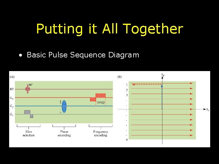
Frequency Encoding • Use a gradient to modify the rate at which the protons spin based on location of the proton • Requires the gradient to remain on

Uniform Field Col 1 Col 2 Col 3 Uniform Field Prior to Gradient

Lower Field Col 1 Col 2 Col 3 Higher Field Gradient Applied

Frequency Encoding • Apply gradient in one direction and leave it on • Result: ØProtons that experience a decrease in the net magnetic field precess slower ØProtons that experience an increase in the net magnetic field precess faster

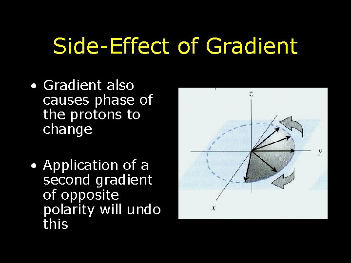
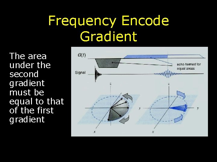
Side-Effect of Gradient • Gradient also causes phase of the protons to change • Application of a second gradient of opposite polarity will undo this

Frequency Encode Gradient The area under the second gradient must be equal to that of the first gradient

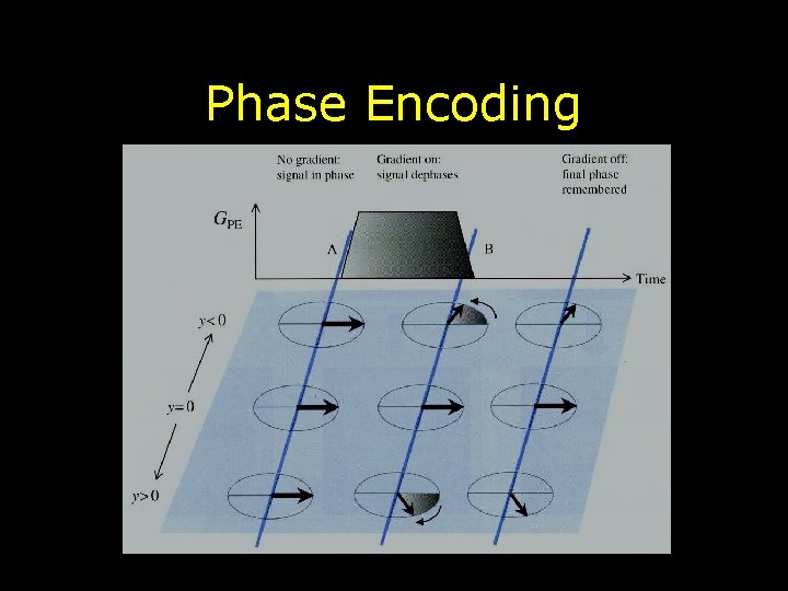
Phase Encoding • Turn gradient on briefly then turn it off • Turning on the gradient will cause some protons to spin faster others to spin slower depending on where they are located • Turning off the gradient will make them all spin at the same rate again • BUT they will be out of ‘phase’ with one another based on where they are located

Phase Encoding

Uniform Field Row 1 Row 2 Row 3 Uniform Field Prior to Gradient

Lower Field Row 1 Row 2 Row 3 Higher Field Gradient Applied

Uniform Field Row 1 Row 2 Row 3 Uniform Field Gradient Turned Off

Phase Encoding • Apply gradient in one direction briefly and then turn off • Result: Ø Protons initially decrease or increase their rate of precession Ø After the gradient is turned off all of the protons will again precess at the same rate Ø Difference is that they will be out phase with one another

Combining Phase & Frequency Encoding Row 1, Col 1 Row 2, Col 2 Row 3, Col 3

Sum Corresponds to Received Signal Row 1, Col 1 Row 2, Col 2 Row 3, Col 3 + +

Converting Received Signal into an Image • Signal produced using both frequency and phase encoding can be decomposed using a mathematical technique called the Inverse Fourier Transform • Result is the signal (sinusoidal squiggles) produced at each individual pixel

Row 1, Col 1 Row 2, Col 2 Row 3, Col 3 From Signal to Image Inv FFT Pixels

Lauterbur’s Insight • Use of gradients to provide spatial encoding • Frequency and Phase - was Lauterbur’s contribution • Awarded Nobel prize for this work

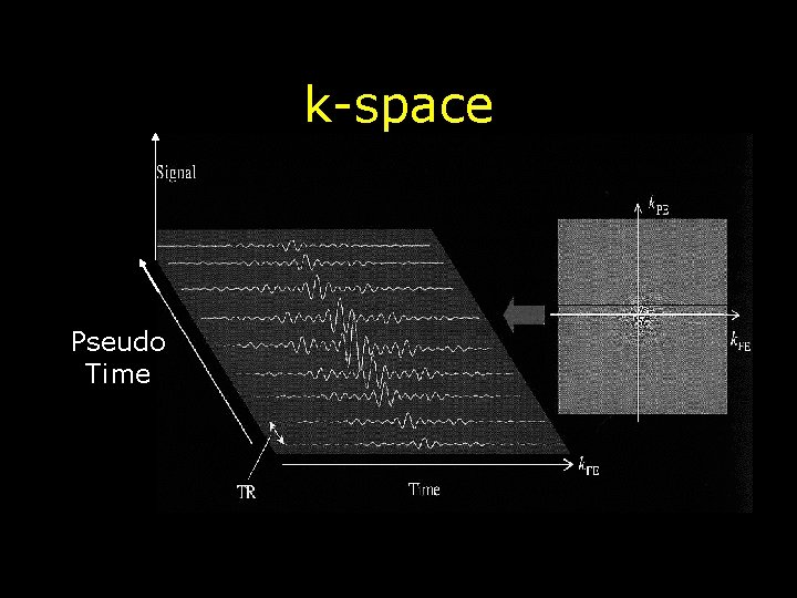
k-space Pseudo Time

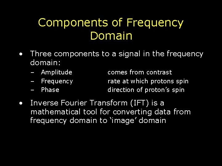
Components of Frequency Domain • Three components to a signal in the frequency domain: – – – Amplitude Frequency Phase comes from contrast rate at which protons spin direction of proton’s spin • Inverse Fourier Transform (IFT) is a mathematical tool for converting data from frequency domain to ‘image’ domain

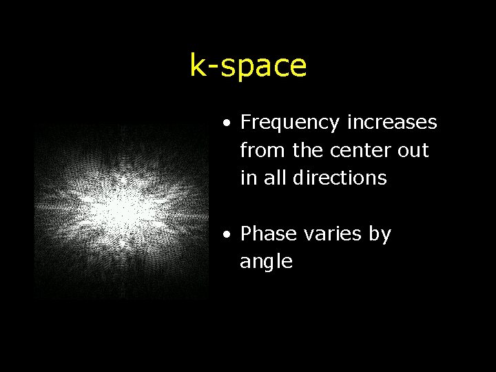
k-space • Frequency increases from the center out in all directions • Phase varies by angle

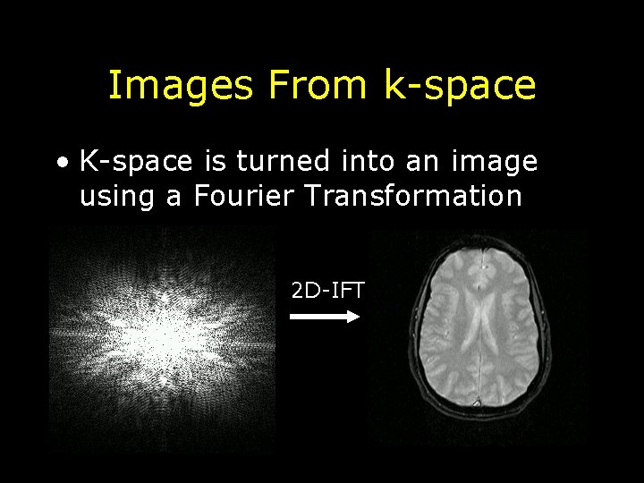
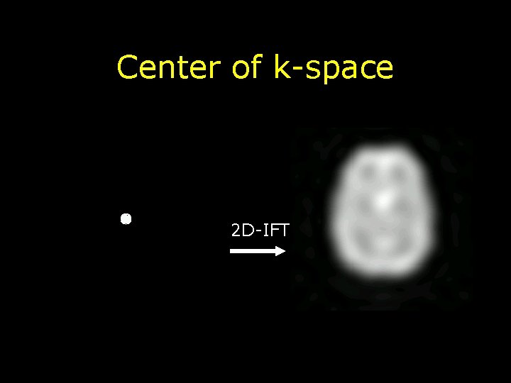
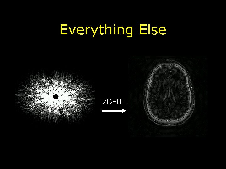
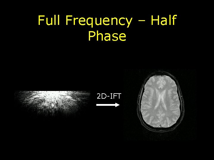
Images From k-space • K-space is turned into an image using a Fourier Transformation 2 D-IFT

Center of k-space 2 D-IFT

Everything Else 2 D-IFT

Full Frequency – Half Phase 2 D-IFT

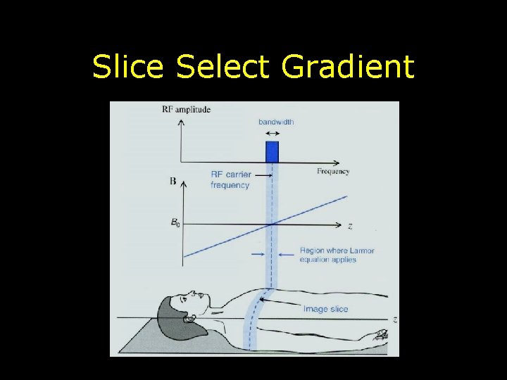
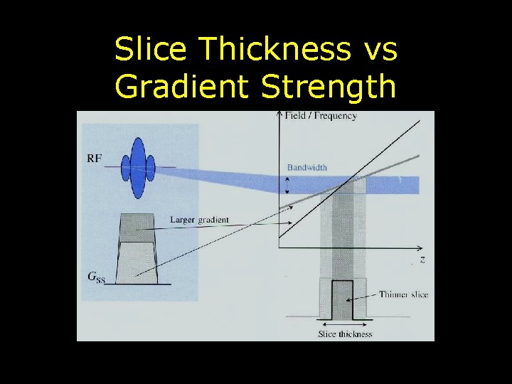
Selecting a Slice • Again use gradient to modify frequency of the proton’s spin • Slice select gradient is positive on one side of the slice and negative on the other side • At the desired slice location the slice select gradient is zero • Thus, protons in this slice and only this slice will be spinning at the center frequency of the scanner! • If this gradient is on when we apply RF pulse only protons in the slice will be tipped into x-y plane and thus measurable

Slice Select Gradient

Slice Thickness vs Gradient Strength

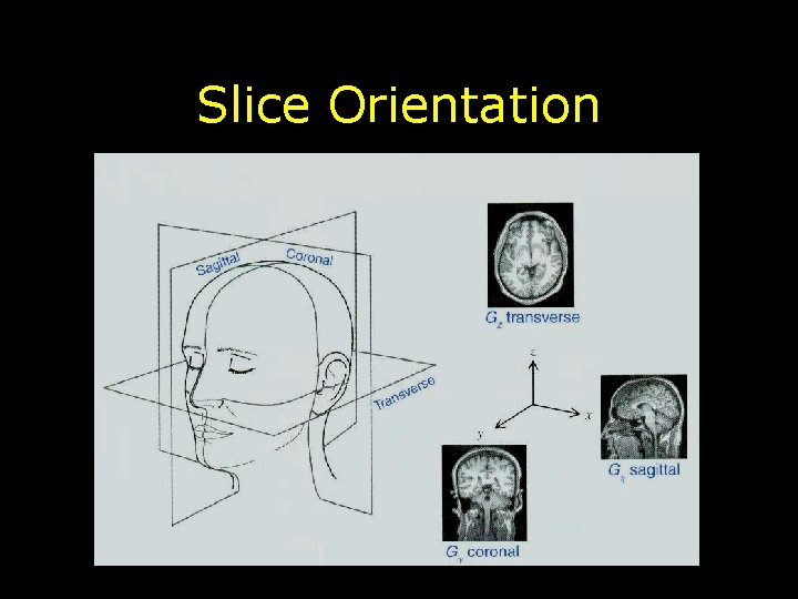
Slice Orientation

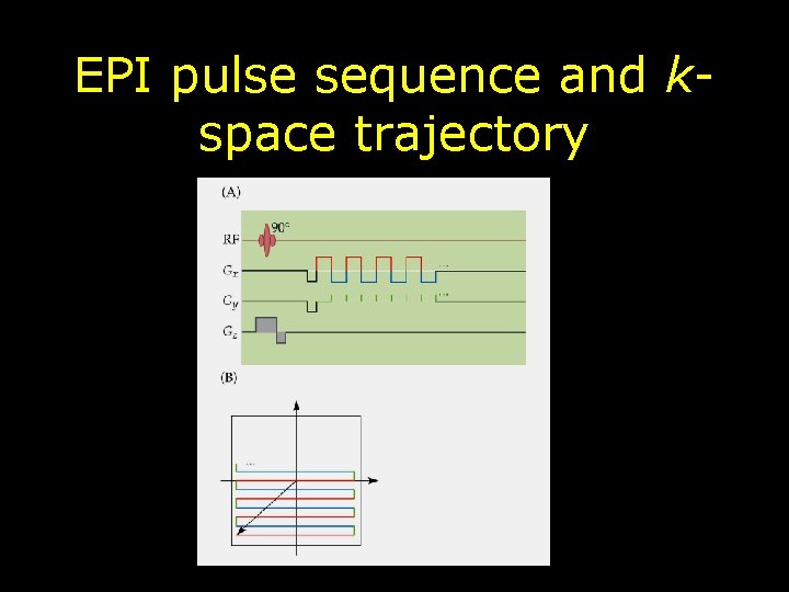
Putting it All Together • Basic Pulse Sequence Diagram

EPI pulse sequence and kspace trajectory

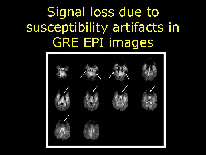
Signal loss due to susceptibility artifacts in GRE EPI images

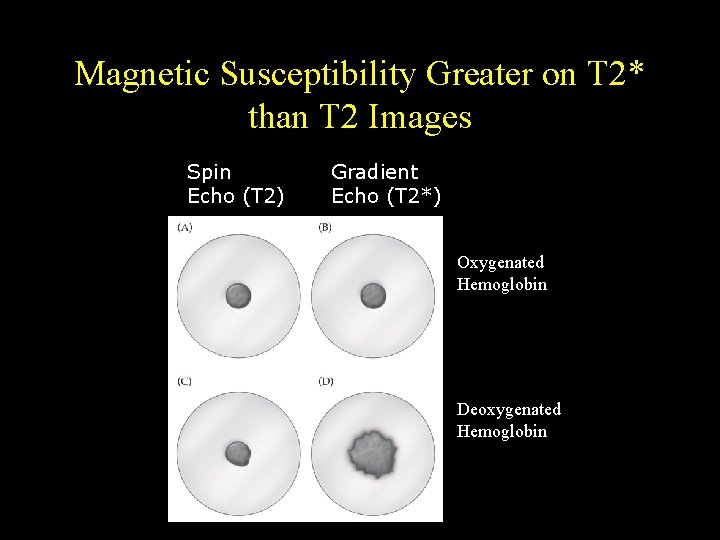
Magnetic Susceptibility Greater on T 2* than T 2 Images Spin Echo (T 2) Gradient Echo (T 2*) Oxygenated Hemoglobin Deoxygenated Hemoglobin

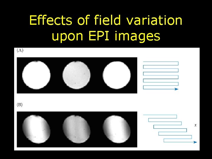
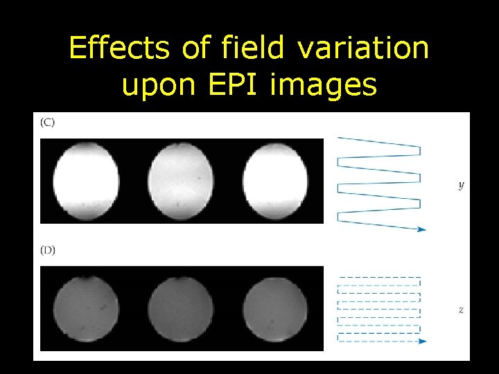
Effects of field variation upon EPI images

Effects of field variation upon EPI images

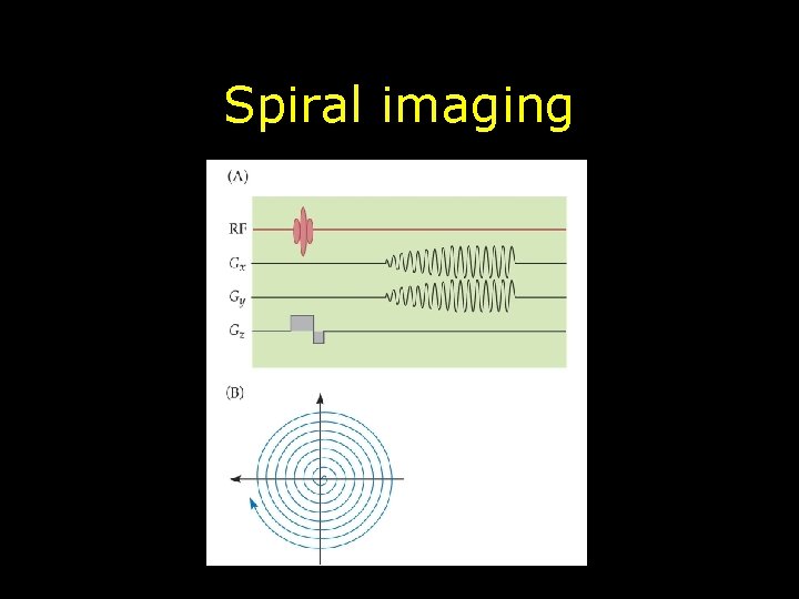
Spiral imaging

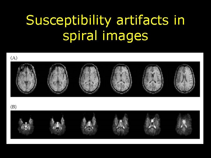
Susceptibility artifacts in spiral images

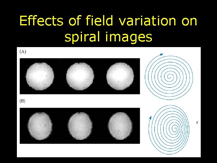
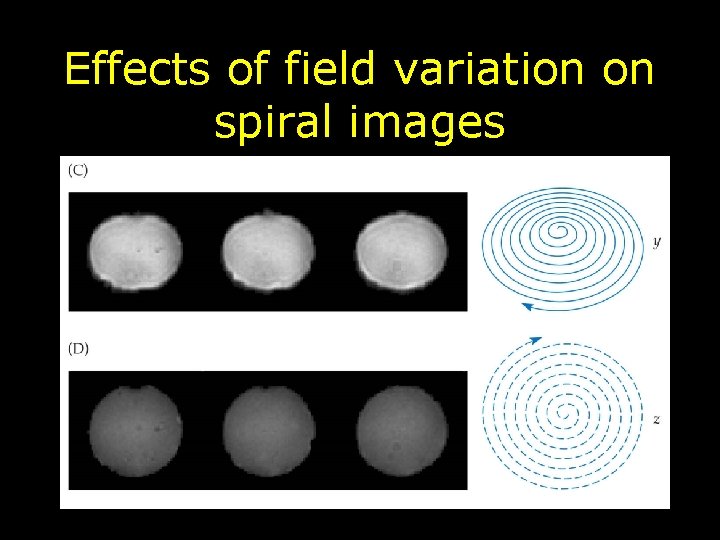
Effects of field variation on spiral images

Effects of field variation on spiral images

Acquisition Matrix Size 64 x 64 Matrix 64 x 128 Matrix Isotropic (square) Anisotropic (oblong) Isotropic (square) Relative SNR = 1 Relative SNR = 0. 5 Relative SNR = 0. 25

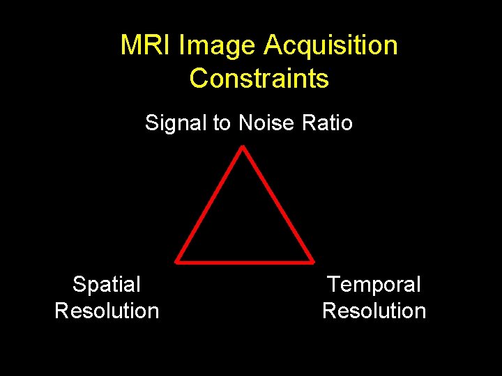
MRI Image Acquisition Constraints Signal to Noise Ratio Spatial Resolution Temporal Resolution