Principles of Programming Languages Type Inference Implementations Review

Principles of Programming Languages Type Inference Implementations

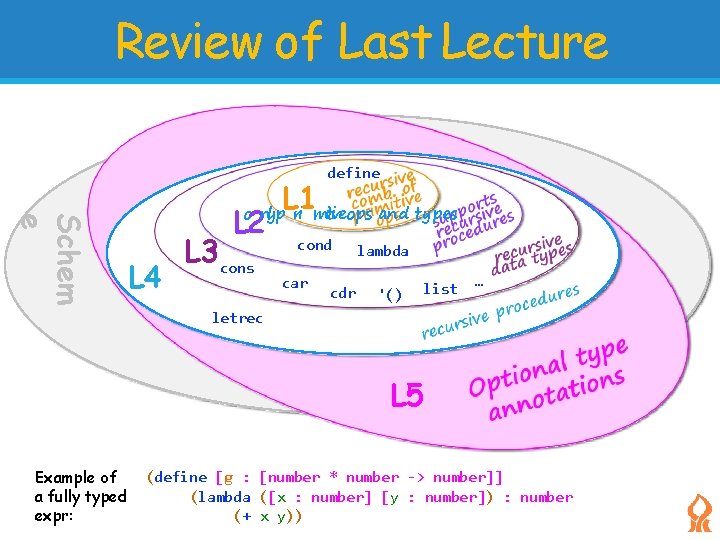
Review of Last Lecture Schem e L 1 define o nlyp ri mitiveops and types L 2 L 4 L 3 cons cond car cdr lambda '() list … letrec L 5 Example of a fully typed expr: (define [g : [number * number -> number]] (lambda ([x : number] [y : number]) : number (+ x y))

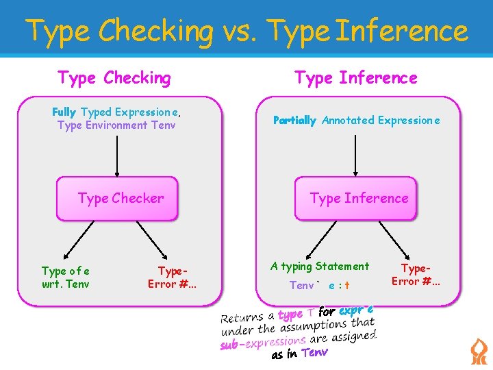
Type Checking vs. Type Inference Type Checking Type Inference Fully Typed Expression e, Type Environment Tenv Partially Annotated Expression e Type Checker Type of e wrt. Tenv Type. Error #. . . Type Inference A typing Statement Tenv ` e : t Type. Error #. . .

Implementation of Type inference Lets talk implementations… Two implementations: 1. One “Literal” application of the algorithm. 2. An optimized algorithm with less traversals of the program.

Implementation of Type inference Lets talk implementations… Two implementations: 1. One “Literal” application of the algorithm. 2. An optimized algorithm with less traversals of the program.

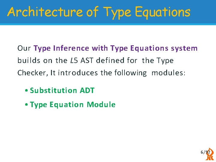
Architecture of Type Equations Our Type Inference with Type Equations system builds on the L 5 AST defined for the Type Checker, It introduces the following modules: • Substitution ADT • Type Equation Module 6/ 92

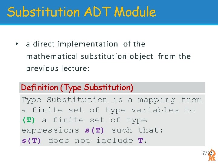
Substitution ADT Module • a direct implementation of the mathematical substitution object from the previous lecture: Definition (Type Substitution) Type Substitution is a mapping from a finite set of type variables to (T) a finite set of type expressions s(T) such that: s(T) does not include T. 7/ 92

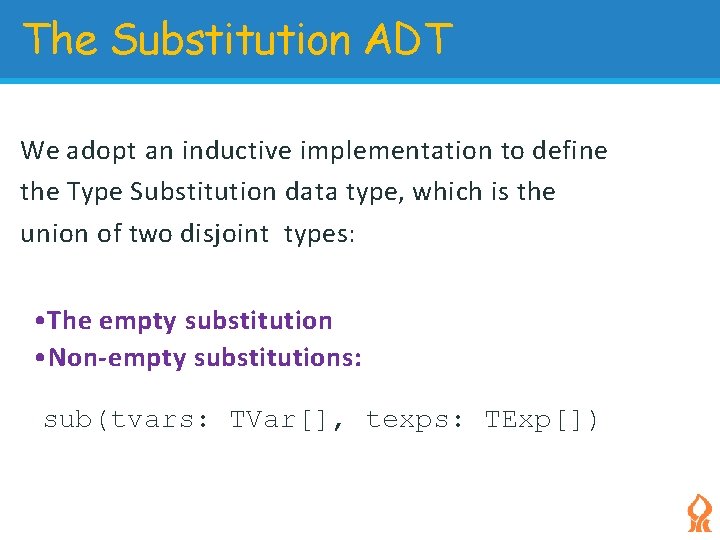
The Substitution ADT We adopt an inductive implementation to define the Type Substitution data type, which is the union of two disjoint types: • The empty substitution • Non-empty substitutions: sub(tvars: TVar[], texps: TExp[])

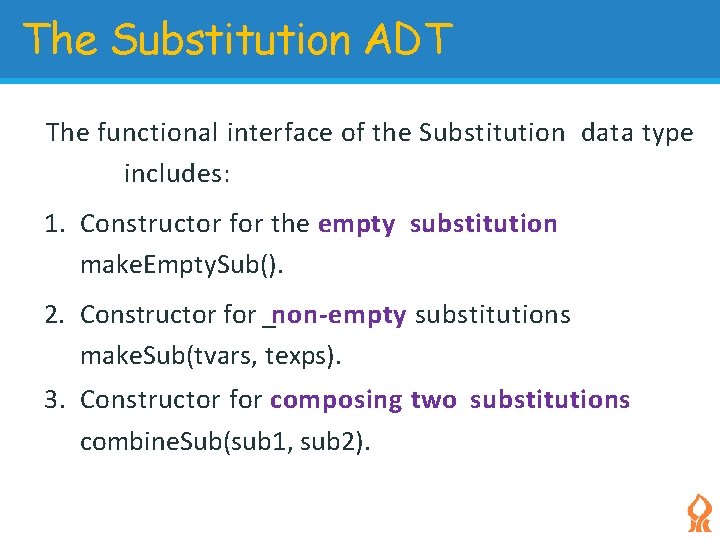
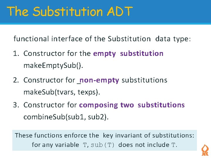
The Substitution ADT The functional interface of the Substitution data type includes: 1. Constructor for the empty substitution make. Empty. Sub(). 2. Constructor for _non-empty substitutions make. Sub(tvars, texps). 3. Constructor for composing two substitutions combine. Sub(sub 1, sub 2).

The Substitution ADT functional interface of the Substitution data type: 1. Constructor for the empty substitution make. Empty. Sub(). 2. Constructor for _non-empty substitutions make. Sub(tvars, texps). 3. Constructor for composing two substitutions combine. Sub(sub 1, sub 2). These functions enforce the key invariant of substitutions: for any variable T, sub(T) does not include T.

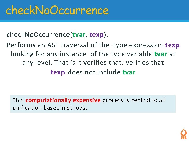
check. No. Occurrence(tvar, texp). Performs an AST traversal of the type expression texp looking for any instance of the type variable tvar at any level. That is it verifies that: verifies that texp does not include tvar This computationally expensive process is central to all unification based methods.

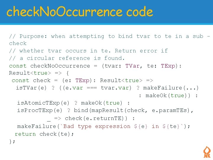
check. No. Occurrence code // Purpose: when attempting to bind tvar to te in a sub check // whether tvar occurs in te. Return error if // a circular reference is found. const check. No. Occurrence = (tvar: TVar, te: TExp): Result<true> => { const check = (e: TExp): Result<true> => is. TVar(e) ? ((e. var === tvar. var) ? make. Failure(. . . ) : make. Ok(true)) : is. Atomic. TExp(e) ? make. Ok(true) : is. Proc. TExp(e) ? bind(map. Result(check, e. param. TEs), _ => check(e. return. TE)) : make. Failure(`Bad type expression ${e} in ${te}`); return check(te); };

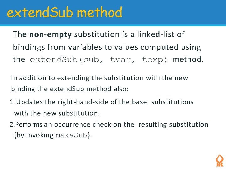
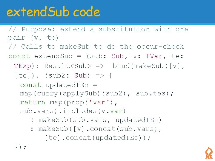
extend. Sub method The non-empty substitution is a linked-list of bindings from variables to values computed using the extend. Sub(sub, tvar, texp) method. In addition to extending the substitution with the new binding the extend. Sub method also: 1. Updates the right-hand-side of the base substitutions with the new substitution. 2. Performs an occurrence check on the resulting substitution (by invoking make. Sub).

extend. Sub code // Purpose: extend a substitution with one pair (v, te) // Calls to make. Sub to do the occur-check const extend. Sub = (sub: Sub, v: TVar, te: TExp): Result<Sub> => bind(make. Sub([v], [te]), (sub 2: Sub) => { const updated. TEs = map(curry(apply. Sub)(sub 2), sub. tes); return map(prop('var'), sub. vars). includes(v. var) ? make. Sub(sub. vars, updated. TEs) : make. Sub([v]. concat(sub. vars), [te]. concat(updated. TEs)); });

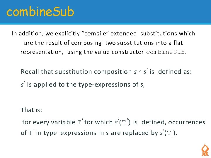
combine. Sub In addition, we explicitly “compile” extended substitutions which are the result of composing two substitutions into a flat representation, using the value constructor combine. Sub. Recall that substitution composition s ◦ s ′ is defined as: s ′ is applied to the type-expressions of s, That is: for every variable T′ for which s ′ (T ′ ) is defined, occurrences of T′ in type expressions in s are replaced by s ′ (T ′ ).

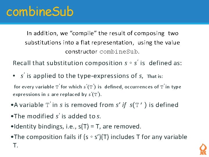
combine. Sub In addition, we “compile” the result of composing two substitutions into a flat representation, using the value constructor combine. Sub. Recall that substitution composition s ◦ s ′ is defined as: • s ′ is applied to the type-expressions of s, That is: for every variable T′ for which s ′ (T ′ ) is defined, occurrences of T′ in type expressions in s are replaced by s ′ (T ′ ). • A variable T′ in s is removed from s’ if s(T’) is defined • The modified s ′ is added to s. • Identity bindings, i. e. , s(T) = T, are removed. • The composition fails if (s ◦ s′)(T) includes T for any variable T.

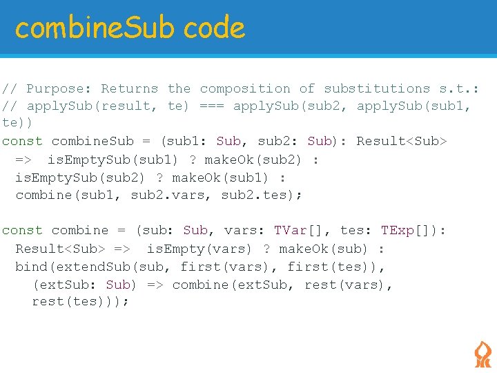
combine. Sub code // Purpose: Returns the composition of substitutions s. t. : // apply. Sub(result, te) === apply. Sub(sub 2, apply. Sub(sub 1, te)) const combine. Sub = (sub 1: Sub, sub 2: Sub): Result<Sub> => is. Empty. Sub(sub 1) ? make. Ok(sub 2) : is. Empty. Sub(sub 2) ? make. Ok(sub 1) : combine(sub 1, sub 2. vars, sub 2. tes); const combine = (sub: Sub, vars: TVar[], tes: TExp[]): Result<Sub> => is. Empty(vars) ? make. Ok(sub) : bind(extend. Sub(sub, first(vars), first(tes)), (ext. Sub: Sub) => combine(ext. Sub, rest(vars), rest(tes)));

Type Equation Module The type equations module follows the type inference algorithm: 1. 2. 3. 4. Rename bound variables in the expression. Assign type variables to all sub-expressions. Construct type equations. Solve the equations.

Step 1: Renaming of all bound variables in e is very similar to the renaming done in the Substitution Model for Operational semantics. We do not repeat this code here. Instead, we assume that all bound variables have distinct names (the same variable name is never used twice in different scopes).

Step 2: Assign Type Variables We define the pool data structure which contains a list of pairs (exp, TVar) for every node in the expression AST. The pool exhaustively includes all the sub-expressions in the AST. It is built using the function exp. To. Pool. Whenever a node in the AST is visited, exp. To. Pool allocates a fresh Type Variable for it.

Step 2: Assign Type Variables Pay attention to the way variable declarations and variable references are processed in the pool: The method extend. Pool(exp, pool) maps exp to a fresh type variable (one that was never used before) and adds the mapping to the pool. When we enter a new scope in the expression (during its traversal), we need to keep track of the variable declarations - and map the variable name to the type of the variable declaration.

Step 2: Assign Type Variables Pay attention to the way variable declarations and variable references are processed in the pool: The method extend. Pool(exp, pool) maps exp to a fresh type variable (one that was never used before) and adds the mapping to the pool. When we enter a new scope in the expression (during its traversal), we need to keep track of the variable declarations - and map the variable name to the type of the variable declaration.

Step 3: The Equation Module Recall that when we parse an L 5 expression, we consider type annotations optional. If they are provided, the Var. Declnode stores the declared type expression in the Var. Decl. texp field. If they are not provided, the parser generates a new fresh variable and associates it to Var. Decl. texp.

Step 3: The Equation Module As we traverse the AST , we associate Var. Ref nodes with corresponding Var. Declnodes. More precisely, when we meet a Var. Decl node, we use the procedure extend. Pool. Var. Decl(var. Decl, pool)which adds the pair (Var. Ref(var. Decl. var), var. Decl. texp) to the pool. When we later reach a Var. Ref in the scope of this Var. Decl, we find that the pair (Var. Ref tvar)already exists in the pool, and we do not allocate a new type variable.

Step 3: The Equation Module This mechanism crucially depends on the fact that exp. To. Pool traverses the expression AST top-down (traverse the Var. Decl before the corresponding Var. Ref nodes are met) and the expression has been renamed before so that all Var. Refs with a given name refer to the single Var. Decl with the same name.

Step 3: The Equation Module exp. To. Pool uses the function reduce. Pool to accumulate the pairs (AST-node, TVar) into the pool without repetitions. This function is a variant of the reduce family of higherorder functions. The in. Pool function checks whether an expression is already present in the pool. If it is, it returns the associated TExp, else we need to return a value that indicates the expression was not found. This is a typical situation where we have a search operator which can fail.

Step 3: The Equation Module We adopt the standard Optional generic type to represent this return type in a type-safe manner. In the same way as Result represents a call which may fail, Optional represents a call which may either return a value or the legitimate case of a missing value (which should not be considered an error). The two options are wrapped as Some<T> and None (parallel to Ok<T> and Failure for Result<T>).

Step 3: The Equation Module To manipulate Optional values, we use the maybe operator which passes the Optional<T> two possible continuations: a method receiving a T value in case the value was found, and one receiving no argument in case none was found. maybe allows type-safe composition of functions returning Optional<T> values in the same way as bind allows typesafe composition of Result<T> values. We also implement bind and safe 2 versions for Optional<T> values with the same behavior as that we adopted for Result<T>.

Step 3: The Equation Module exp. To. Pool code can be found here. The post-condition met at the end of the pool construction is that every node in the AST is mapped to a type variable while preserving scoping relations (different occurrences of the same Var. Ref are all merged as a single pair mapping the Var. Ref to its declared type - which can be a noninstantiated type variable).

Step 3: The Equation Module Finally, we generate the equations by transforming the pool of{e: exp, te: TVar}pairs into a set of equations. This part of the algorithm encapsulates the semantics of the type system. The procedure pool. To. Equations performs this mapping. It accumulates the transformation of all pairs in the pool to equations. The equation ADT is a pair left-hand-side / right-hand-side of type expressions{left: TExp, right: TExp}).

Step 3: The Equation Module The heart of the typing algorithm is the operation make. Equations. From. Exp which covers the typing rules of the programming language. This implements the typing rules for procedure expressions, application expressions and atomic expressions. For example, given a pair (app-exp, TVar), the procedure derives a type equation which mandates that the type variable associated to the operator of the application must be made equal to the type expression.

Step 3: The Equation Module For the base cases of primitive operators, we reuse the procedure typeof. Prim which we defined in the type checker. Observe that there is no processing of if expressions do you understand why?

Step 4: Solving the equations The procedure solve(equations, substitution) is a direct implementation of the solve algorithm presented in the last lecture. It computes the unifier of all the equations - that is, it computes a type substitution that makes both sides of all equations equal when applied. This unifier substitution is computed incrementally, by processing each equation in turn.

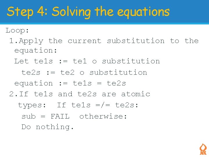
Step 4: Solving the equations Reminder of the algorithm from last lecture: Input: A set of type equations. Output: A type substitution or FAIL. Initialization: 1. substitution : = { } 2. Order the set of input equations in any sequential order. 3. equation : = te 1 = te 2, the first equation.

Step 4: Solving the equations Loop: 1. Apply the current substitution to the equation: Let te 1 s : = te 1 o substitution te 2 s : = te 2 o substitution equation : = te 1 s = te 2 s 2. If te 1 s and te 2 s are atomic types: If te 1 s =/= te 2 s: sub = FAIL otherwise: Do nothing.

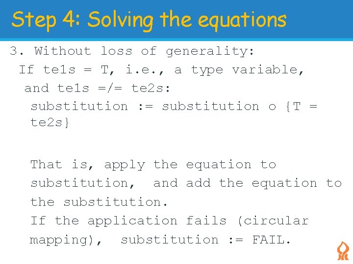
Step 4: Solving the equations 3. Without loss of generality: If te 1 s = T, i. e. , a type variable, and te 1 s =/= te 2 s: substitution : = substitution o {T = te 2 s} That is, apply the equation to substitution, and add the equation to the substitution. If the application fails (circular mapping), substitution : = FAIL.

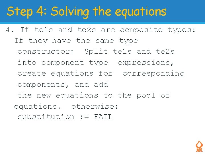
Step 4: Solving the equations 4. If te 1 s and te 2 s are composite types: If they have the same type constructor: Split te 1 s and te 2 s into component type expressions, create equations for corresponding components, and add the new equations to the pool of equations. otherwise: substitution : = FAIL

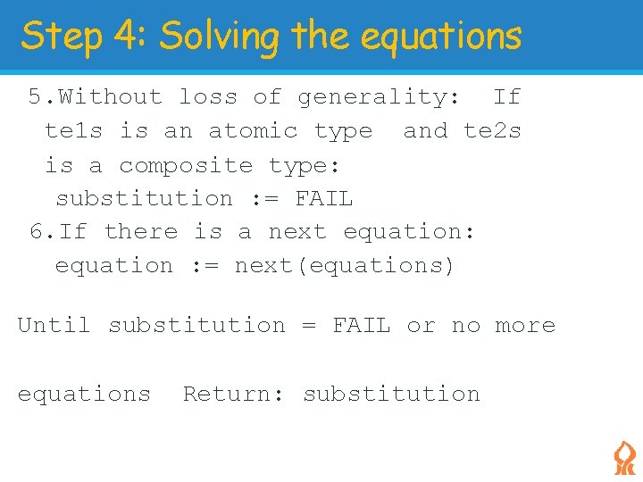
Step 4: Solving the equations 5. Without loss of generality: If te 1 s is an atomic type and te 2 s is a composite type: substitution : = FAIL 6. If there is a next equation: equation : = next(equations) Until substitution = FAIL or no more equations Return: substitution

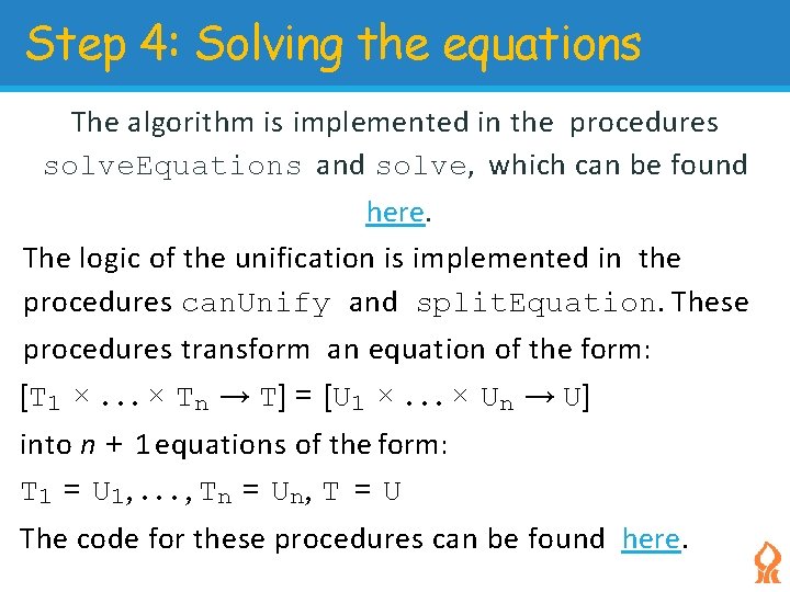
Step 4: Solving the equations The algorithm is implemented in the procedures solve. Equations and solve, which can be found here. The logic of the unification is implemented in the procedures can. Unify and split. Equation. These procedures transform an equation of the form: [T 1 ×. . . × Tn → T] = [U 1 ×. . . × Un → U] into n + 1 equations of the form: T 1 = U 1 , . . . , Tn = U n , T = U The code for these procedures can be found here.

Step 4: Solving the equations How do we know that the solve algorithm terminates given a list of type expression equations? The main loop of the algorithm has for state the current list of equations and the current substitution.

Step 4: Solving the equations Let us consider the effect of one iteration through the main loop: Either we consume one equation from the current equations set and produce a more complex substitution (this happens when one of the sides of the first equation is an atomic type expression or a type variable).

Step 4: Solving the equations Or we replace one equation with multiple equations: this happens when both sides of the equation are composite type expressions with compatible structure. In this case, we replace one equation with AST trees of depth D with n equations of depth D − 1 where n is the number of children of the ASTs.

Step 4: Solving the equations In our case, composite ASTs in the type language are Proc. TExp nodes which represent the type of procedures - with n children elements for the arguments of the procedure and one element for the return type. Or we fail the solve process when we detect an incompatible equation.

Step 4: Solving the equations The argument for completion is based on the characterization of the size of the input equation set as a pair (D, N) where D is the maximum height of the ASTs that appear in any equation in the equation set and N is the number of equations in the set.

Step 4: Solving the equations Each iteration in the loop changes the size to either (D, N − 1) or (D − 1, N + n). When D = 1, the transition is necessarily to (1, N − 1) because the only case where we add equations is for composite ASTs. Hence all transitions lead to the completion state of (1, 0). Putting all the steps of the algorithm together, we define the procedures infer and infer. Type. See the code here.

Putting it all together: Example: infer("(lambda (f g) (lambda (n) (f (g n))))"); // { tag: 'Ok', // value: '((T_6 -> T_7) * (T_3 -> T_6) -> (T_3 -> T_7))' } Observe the usage of freshly generated type variable names which are different each time we invoke the procedure. This makes it difficult to test the procedure.

Putting it all together: To resolve this difficulty, we introduce the procedure equivalent. TEs in TExp. ts which verifies that two type expressions are equivalent up to type variable renaming. This allows us to write tests in a deterministic manner (see here).

Putting it all together: To resolve this difficulty, we introduce the procedure equivalent. TEs in TExp. ts which verifies that two type expressions are equivalent up to type variable renaming. This allows us to write tests in a deterministic manner (see here).

Putting it all together: The implementation described above based on type equations follows literally the type equations algorithm. It explicitly manipulates substitution data structures and type equations. In addition, it constructs a map of expression to type variables to ensure the exhaustive traversal of the program.

Next Lecture An optimized algorithm with less traversals of the program.

Next Lecture An optimized algorithm with less traversals of the program.

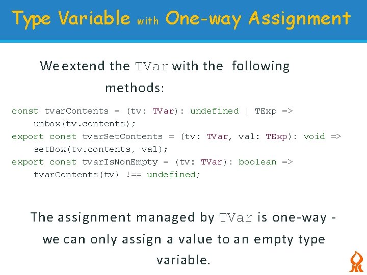
Type Variable with One-way Assignment We extend Tvar to be initially initialized to undefined using the box interface. We require this extension as we do not have a type when we first encounter Tvar. During type inference we will bind Tvar to a type (as more constraints appear).

Type Variable with One-way Assignment We extend the TVar with the following methods: const tvar. Contents = (tv: TVar): undefined | TExp => unbox(tv. contents); export const tvar. Set. Contents = (tv: TVar, val: TExp): void => set. Box(tv. contents, val); export const tvar. Is. Non. Empty = (tv: TVar): boolean => tvar. Contents(tv) !== undefined; The assignment managed by TVar is one-way we can only assign a value to an empty type variable.

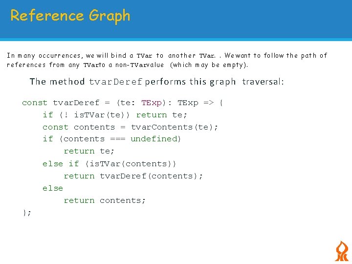
Reference Graph I n m a n y occurrences, we will b i n d a TVar to a n o t h e r TVar. . We want to follow the p a t h of references from a n y TVarto a non-TVarv a l u e (which m a y b e empty). The method tvar. Deref performs this graph traversal: const tvar. Deref = (te: TExp): TExp => { if (! is. TVar(te)) return te; const contents = tvar. Contents(te); if (contents === undefined) return te; else if (is. TVar(contents)) return tvar. Deref(contents); else return contents; };

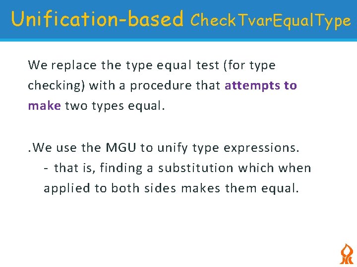
Unification-based Check. Tvar. Equal. Type We replace the type equal test (for type checking) with a procedure that attempts to make two types equal. . We use the MGU to unify type expressions. - that is, finding a substitution which when applied to both sides makes them equal.

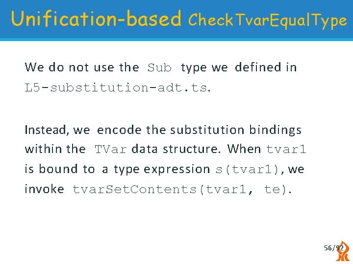
Unification-based Check. Tvar. Equal. Type We do not use the Sub type we defined in L 5 -substitution-adt. ts. Instead, we encode the substitution bindings within the TVar data structure. When tvar 1 is bound to a type expression s(tvar 1), we invoke tvar. Set. Contents(tvar 1, te). 56/ 92

Unification-based Check. Tvar. Equal. Type The check. TVar. Equal. Types procedure binds a TVar to a value – a n d e n f o r c e s t h a t t h e r e a r e n o c i r c u l a r references Surprisingly, the type inference algorithm is the same code as the Type Checker - except for the transformation of the procedure check. Equal. Type from a test of equality to the unification building version presented above. 57/ 92

Type Inference Algorithm 2. Each time an application or procedure node is encountered, the corresponding type equation is verified, and solved in place by invoking check. Equal. Type eagerly. Note that the types may not yet be known, and an expression may still be attached to an unbound TVar. This happens for example when we infer types for the expression((lambda (x) x) 1) – when the operator component of this application is analyzed - there is not sufficient information to derive the type of the parameter 58/ 92 x.

Type Inference Algorithm Later, when the typing rule of the application syntactic construct is applied (the top level node in the AST), the TVar associated to x will be bound to the type expression of the numeric atomic value. This will propagate the inferred information that x is a Num. TExp type from the application to the procedure expression. 59/ 92

Type Inference Algorithm This propagation of information was not necessary in the case of the type checking algorithm because we could rely on the fact that all variable references (Var. Ref) are explicitly typed. 60/ 92

Summary 1. No explicit substitution representation. We do not explicitly represent substitutions, instead we rely on the graph of TVar references as a representation of the substitution object. 61/ 92

Summary 2. No renaming of the program (we use Tenv). We do not need the explicit renaming of the program as we can rely on the TEnv mechanism to capture scoping relations. 62/ 92

Summary 3. Unification by One-way Variable Assignment The implementation of unification through one-way variable assignment is a powerful technique, which we will revisit in Chapter 5 when we survey Logic Programming. 63/ 92