PRINCIPLES OF MICROECONOMICS Chapter 5 Elasticity Power Point

PRINCIPLES OF MICROECONOMICS Chapter 5 Elasticity Power. Point Image Slideshow This Open. Stax ancillary resource is © Rice University under a CC-BY 4. 0 International license; it may be reproduced or modified but must be attributed to Open. Stax, Rice University and any changes must be noted. Any images credited to other sources are similarly available for reproduction, but must be attributed to their sources.

FIGURE 5. 1 Netflix, Inc. is an American provider of on-demand Internet streaming media to many countries around the world, including the United States, and of flat rate DVD-by-mail in the United States. (Credit: modification of work by Traci Lawson/Flickr Creative Commons) This Open. Stax ancillary resource is © Rice University under a CC-BY 4. 0 International license; it may be reproduced or modified but must be attributed to Open. Stax, Rice University and any changes must be noted. Any images credited to other sources are similarly available for reproduction, but must be attributed to their sources.

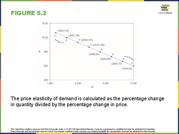
FIGURE 5. 2 The price elasticity of demand is calculated as the percentage change in quantity divided by the percentage change in price. This Open. Stax ancillary resource is © Rice University under a CC-BY 4. 0 International license; it may be reproduced or modified but must be attributed to Open. Stax, Rice University and any changes must be noted. Any images credited to other sources are similarly available for reproduction, but must be attributed to their sources.

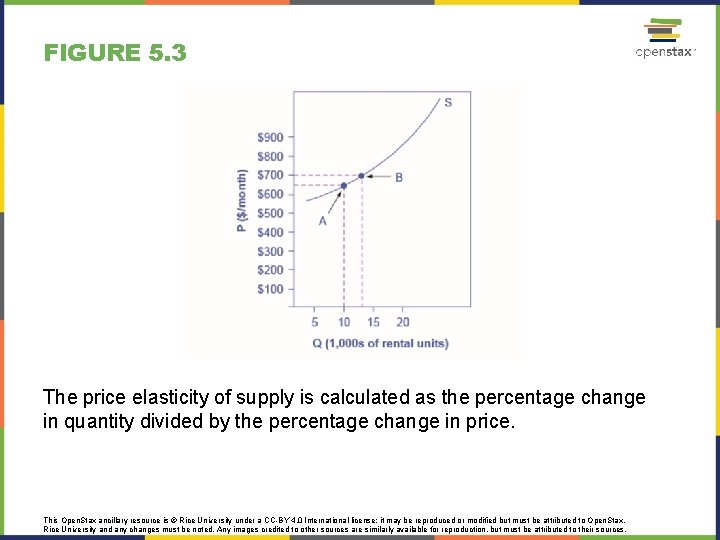
FIGURE 5. 3 The price elasticity of supply is calculated as the percentage change in quantity divided by the percentage change in price. This Open. Stax ancillary resource is © Rice University under a CC-BY 4. 0 International license; it may be reproduced or modified but must be attributed to Open. Stax, Rice University and any changes must be noted. Any images credited to other sources are similarly available for reproduction, but must be attributed to their sources.

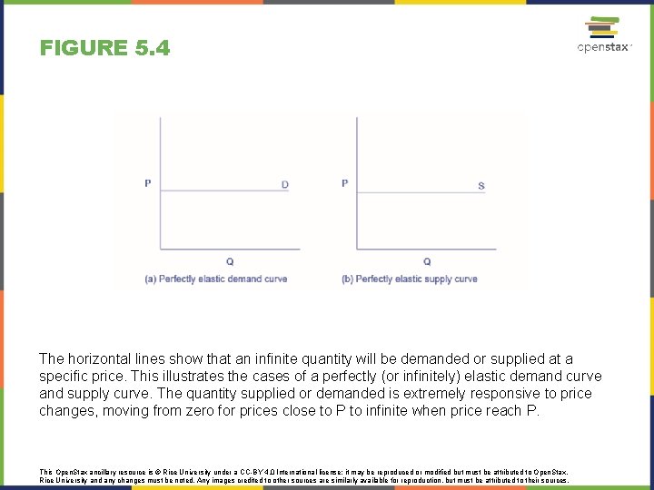
FIGURE 5. 4 The horizontal lines show that an infinite quantity will be demanded or supplied at a specific price. This illustrates the cases of a perfectly (or infinitely) elastic demand curve and supply curve. The quantity supplied or demanded is extremely responsive to price changes, moving from zero for prices close to P to infinite when price reach P. This Open. Stax ancillary resource is © Rice University under a CC-BY 4. 0 International license; it may be reproduced or modified but must be attributed to Open. Stax, Rice University and any changes must be noted. Any images credited to other sources are similarly available for reproduction, but must be attributed to their sources.

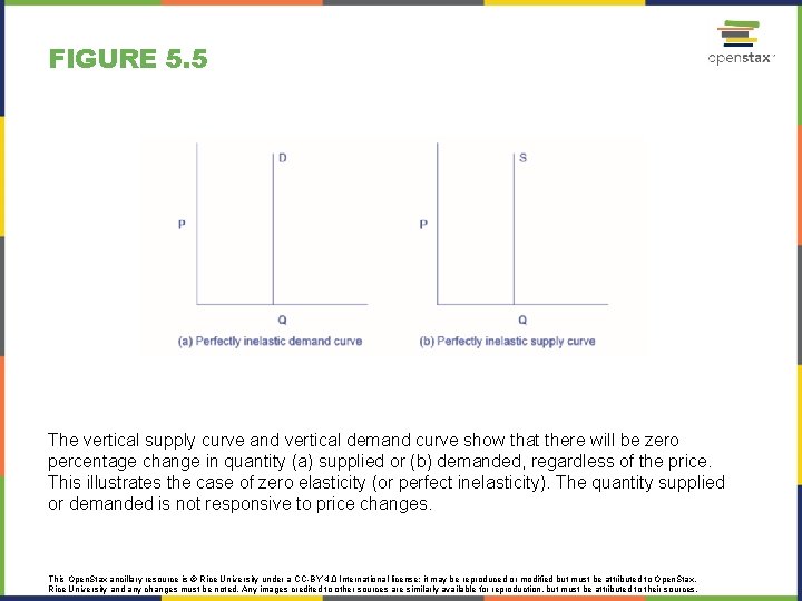
FIGURE 5. 5 The vertical supply curve and vertical demand curve show that there will be zero percentage change in quantity (a) supplied or (b) demanded, regardless of the price. This illustrates the case of zero elasticity (or perfect inelasticity). The quantity supplied or demanded is not responsive to price changes. This Open. Stax ancillary resource is © Rice University under a CC-BY 4. 0 International license; it may be reproduced or modified but must be attributed to Open. Stax, Rice University and any changes must be noted. Any images credited to other sources are similarly available for reproduction, but must be attributed to their sources.

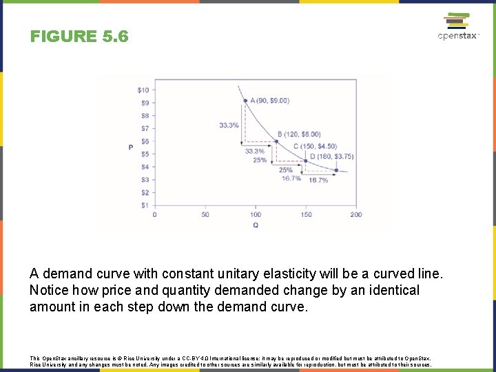
FIGURE 5. 6 A demand curve with constant unitary elasticity will be a curved line. Notice how price and quantity demanded change by an identical amount in each step down the demand curve. This Open. Stax ancillary resource is © Rice University under a CC-BY 4. 0 International license; it may be reproduced or modified but must be attributed to Open. Stax, Rice University and any changes must be noted. Any images credited to other sources are similarly available for reproduction, but must be attributed to their sources.

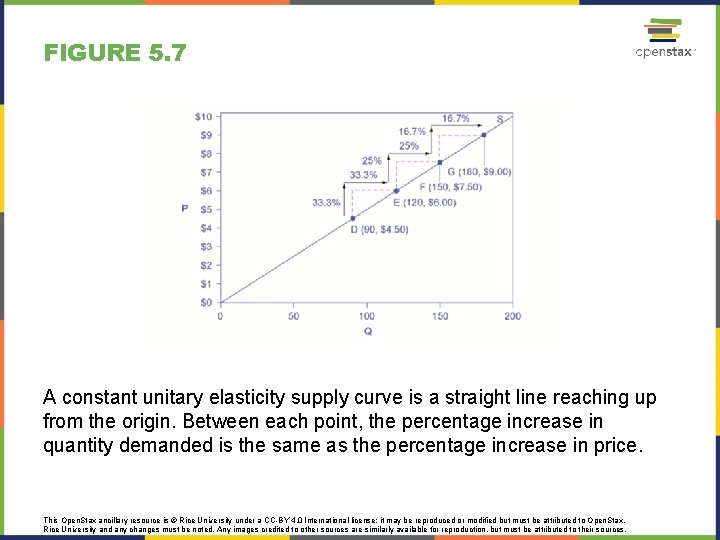
FIGURE 5. 7 A constant unitary elasticity supply curve is a straight line reaching up from the origin. Between each point, the percentage increase in quantity demanded is the same as the percentage increase in price. This Open. Stax ancillary resource is © Rice University under a CC-BY 4. 0 International license; it may be reproduced or modified but must be attributed to Open. Stax, Rice University and any changes must be noted. Any images credited to other sources are similarly available for reproduction, but must be attributed to their sources.

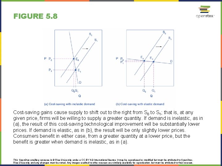
FIGURE 5. 8 Cost-saving gains cause supply to shift out to the right from S 0 to S 1; that is, at any given price, firms will be willing to supply a greater quantity. If demand is inelastic, as in (a), the result of this cost-saving technological improvement will be substantially lower prices. If demand is elastic, as in (b), the result will be only slightly lower prices. Consumers benefit in either case, from a greater quantity at a lower price, but the benefit is greater when demand is inelastic, as in (a). This Open. Stax ancillary resource is © Rice University under a CC-BY 4. 0 International license; it may be reproduced or modified but must be attributed to Open. Stax, Rice University and any changes must be noted. Any images credited to other sources are similarly available for reproduction, but must be attributed to their sources.

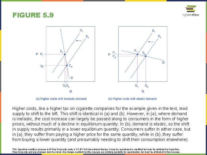
FIGURE 5. 9 Higher costs, like a higher tax on cigarette companies for the example given in the text, lead supply to shift to the left. This shift is identical in (a) and (b). However, in (a), where demand is inelastic, the cost increase can largely be passed along to consumers in the form of higher prices, without much of a decline in equilibrium quantity. In (b), demand is elastic, so the shift in supply results primarily in a lower equilibrium quantity. Consumers suffer in either case, but in (a), they suffer from paying a higher price for the same quantity, while in (b), they suffer from buying a lower quantity (and presumably needing to shift their consumption elsewhere). This Open. Stax ancillary resource is © Rice University under a CC-BY 4. 0 International license; it may be reproduced or modified but must be attributed to Open. Stax, Rice University and any changes must be noted. Any images credited to other sources are similarly available for reproduction, but must be attributed to their sources.

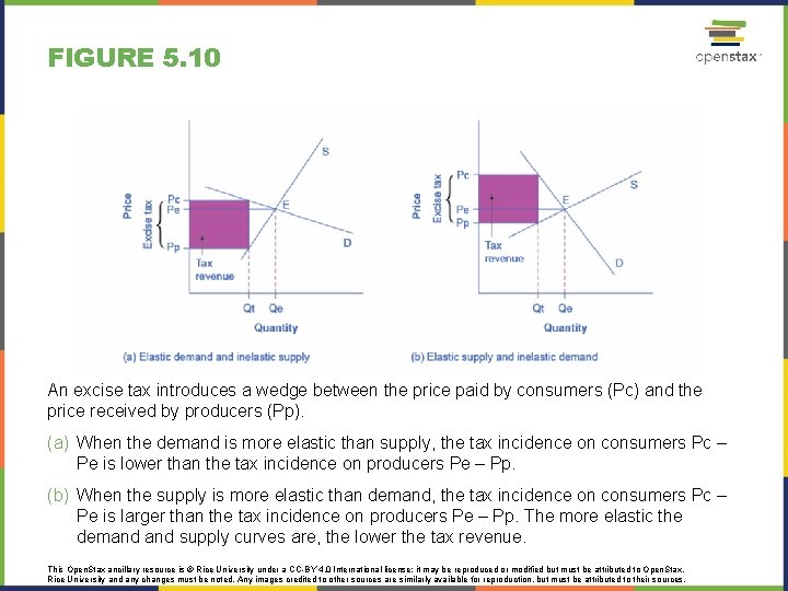
FIGURE 5. 10 An excise tax introduces a wedge between the price paid by consumers (Pc) and the price received by producers (Pp). (a) When the demand is more elastic than supply, the tax incidence on consumers Pc – Pe is lower than the tax incidence on producers Pe – Pp. (b) When the supply is more elastic than demand, the tax incidence on consumers Pc – Pe is larger than the tax incidence on producers Pe – Pp. The more elastic the demand supply curves are, the lower the tax revenue. This Open. Stax ancillary resource is © Rice University under a CC-BY 4. 0 International license; it may be reproduced or modified but must be attributed to Open. Stax, Rice University and any changes must be noted. Any images credited to other sources are similarly available for reproduction, but must be attributed to their sources.

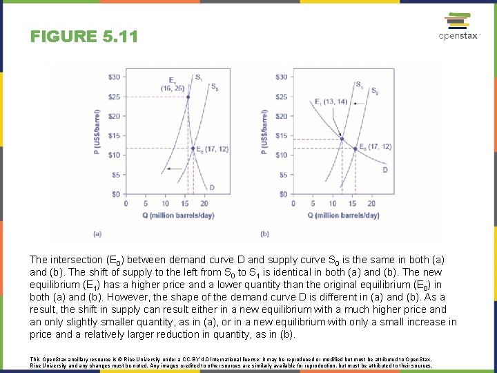
FIGURE 5. 11 The intersection (E 0) between demand curve D and supply curve S 0 is the same in both (a) and (b). The shift of supply to the left from S 0 to S 1 is identical in both (a) and (b). The new equilibrium (E 1) has a higher price and a lower quantity than the original equilibrium (E 0) in both (a) and (b). However, the shape of the demand curve D is different in (a) and (b). As a result, the shift in supply can result either in a new equilibrium with a much higher price and an only slightly smaller quantity, as in (a), or in a new equilibrium with only a small increase in price and a relatively larger reduction in quantity, as in (b). This Open. Stax ancillary resource is © Rice University under a CC-BY 4. 0 International license; it may be reproduced or modified but must be attributed to Open. Stax, Rice University and any changes must be noted. Any images credited to other sources are similarly available for reproduction, but must be attributed to their sources.