Principles of Microeconomics 09 Welfare and Market Efficiency

Principles of Microeconomics 09. Welfare and Market Efficiency* Juan Pablo Chauvin August 4, 2011 * Slide content principally sourced from N. Gregory Mankiw “Principles of Economics” Premium Powe. Point

Contents 1. Review of previous lecture 2. An auction 3. Prices and consumer surplus

1. Review

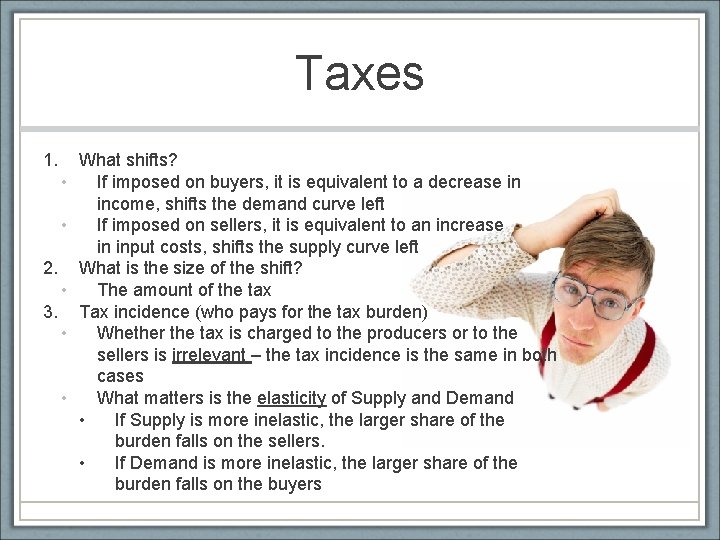
Taxes 1. • • 2. • 3. • • What shifts? If imposed on buyers, it is equivalent to a decrease in income, shifts the demand curve left If imposed on sellers, it is equivalent to an increase in input costs, shifts the supply curve left What is the size of the shift? The amount of the tax Tax incidence (who pays for the tax burden) Whether the tax is charged to the producers or to the sellers is irrelevant – the tax incidence is the same in both cases What matters is the elasticity of Supply and Demand • If Supply is more inelastic, the larger share of the burden falls on the sellers. • If Demand is more inelastic, the larger share of the burden falls on the buyers

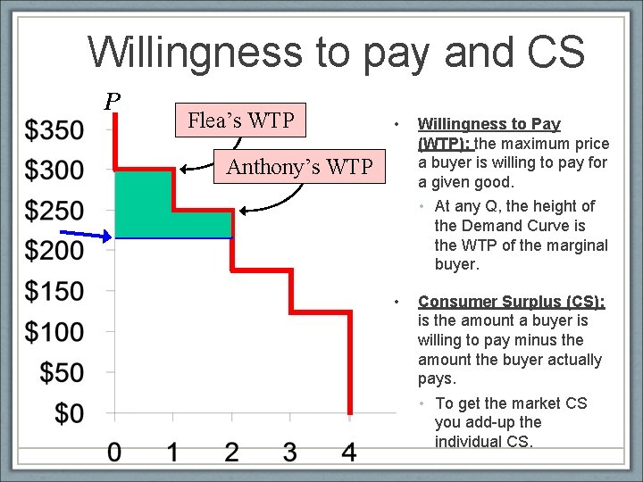
Willingness to pay and CS P Flea’s WTP • Anthony’s WTP Willingness to Pay (WTP): the maximum price a buyer is willing to pay for a given good. • At any Q, the height of the Demand Curve is the WTP of the marginal buyer. • Consumer Surplus (CS): is the amount a buyer is willing to pay minus the amount the buyer actually pays. • To get the market CS you add-up the individual CS.

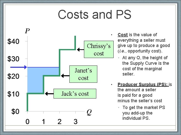
Costs and PS P • Chrissy’s cost • At any Q, the height of the Supply Curve is the cost of the marginal seller. Janet’s cost • Jack’s cost Q Cost is the value of everything a seller must give up to produce a good (i. e. , opportunity cost). Producer Surplus (PS): is the amount a seller is paid for a good minus the seller’s cost • To get the market PS you add-up the individual PS.

2. An auction

Product: Hand-made picture frames

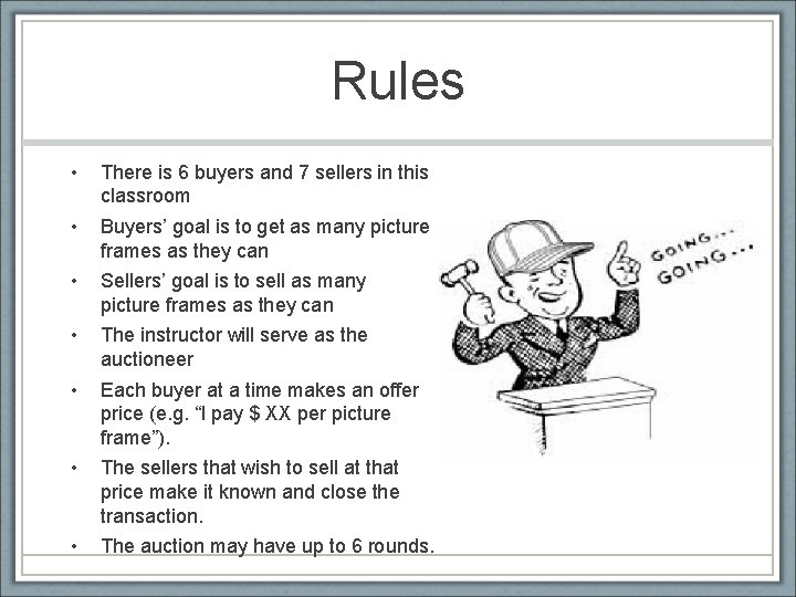
Rules • There is 6 buyers and 7 sellers in this classroom • Buyers’ goal is to get as many picture frames as they can • Sellers’ goal is to sell as many picture frames as they can • The instructor will serve as the auctioneer • Each buyer at a time makes an offer price (e. g. “I pay $ XX per picture frame”). • The sellers that wish to sell at that price make it known and close the transaction. • The auction may have up to 6 rounds.

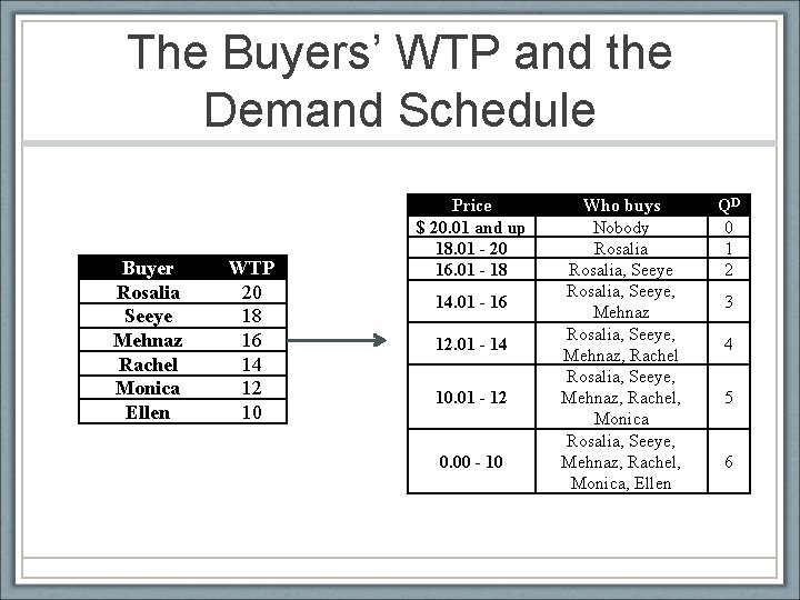
The Buyers’ WTP and the Demand Schedule Buyer Rosalia Seeye Mehnaz Rachel Monica Ellen WTP 20 18 16 14 12 10 Price $ 20. 01 and up 18. 01 - 20 16. 01 - 18 14. 01 - 16 12. 01 - 14 10. 01 - 12 0. 00 - 10 Who buys Nobody Rosalia, Seeye, Mehnaz, Rachel Rosalia, Seeye, Mehnaz, Rachel, Monica, Ellen QD 0 1 2 3 4 5 6

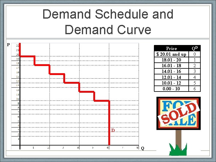
Demand Schedule and Demand Curve P Price $ 20. 01 and up 18. 01 - 20 16. 01 - 18 14. 01 - 16 12. 01 - 14 10. 01 - 12 0. 00 - 10 D Q QD 0 1 2 3 4 5 6

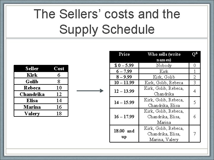
The Sellers’ costs and the Supply Schedule Price Seller Kirk Golib Rebeca Chandrika Elisa Marina Valery Cost 6 8 10 12 14 16 18 $ 0 – 5. 99 6 – 7. 99 8 – 9. 99 10 – 11. 99 12 – 13. 99 14 – 15. 99 16 – 17. 99 18. 00 and up Who sells (write names) Nobody Kirk, Golib, Rebeca, Chandrika Kirk, Golib, Rebeca, Chandrika, Elisa, Marina, Valery QS 0 1 2 3 4 5 6 7

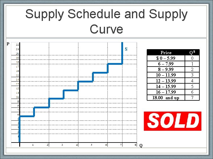
Supply Schedule and Supply Curve P S Price $ 0 – 5. 99 6 – 7. 99 8 – 9. 99 10 – 11. 99 12 – 13. 99 14 – 15. 99 16 – 17. 99 18. 00 and up Q QS 0 1 2 3 4 5 6 7

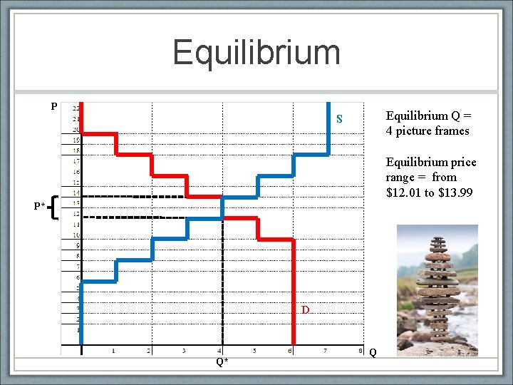
Equilibrium P Equilibrium Q = 4 picture frames S Equilibrium price range = from $12. 01 to $13. 99 P* D Q* Q

3. Prices and Consumer Surplus

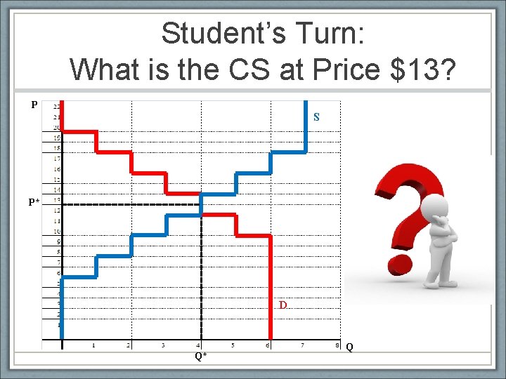
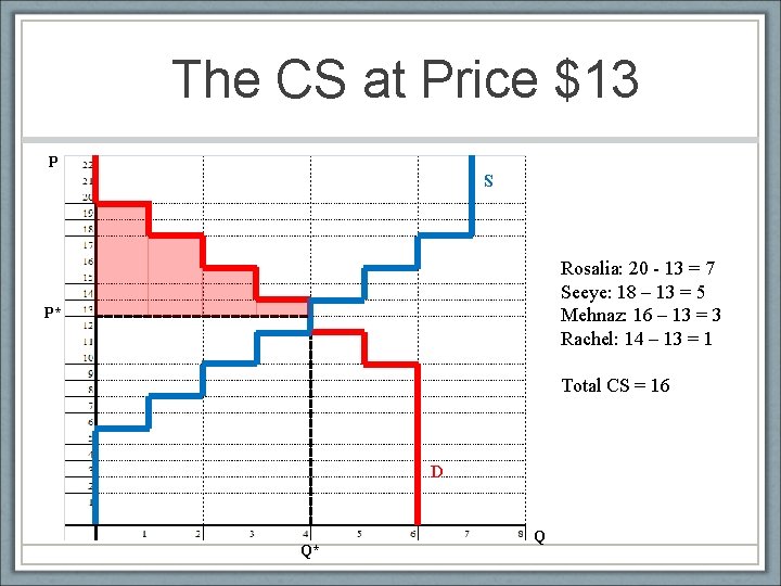
Student’s Turn: What is the CS at Price $13? P S P* D Q* Q

The CS at Price $13 P S Rosalia: 20 - 13 = 7 Seeye: 18 – 13 = 5 Mehnaz: 16 – 13 = 3 Rachel: 14 – 13 = 1 P* Total CS = 16 D Q* Q

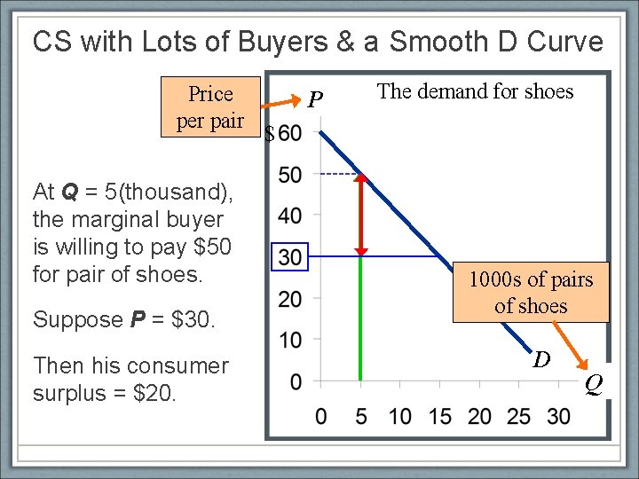
CS with Lots of Buyers & a Smooth D Curve Price per pair At Q = 5(thousand), the marginal buyer is willing to pay $50 for pair of shoes. Suppose P = $30. Then his consumer surplus = $20. P The demand for shoes $ 1000 s of pairs of shoes D Q

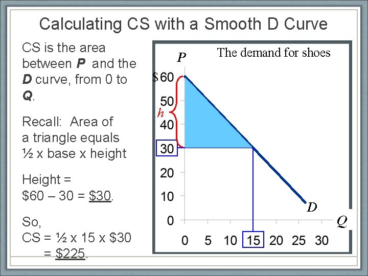
Calculating CS with a Smooth D Curve CS is the area between P and the D curve, from 0 to Q. Recall: Area of a triangle equals ½ x base x height Height = $60 – 30 = $30. So, CS = ½ x 15 x $30 = $225. P The demand for shoes $ h D Q

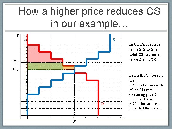
How a higher price reduces CS in our example… P S In the Price raises from $13 to $15, total CS decreases from $16 to $ 9. P*2 P*1 From the $7 loss in CS: • $ 6 are because each of the 3 buyers remaining pays $2 more per frame. • $ 1 is because one buyer left the market D Q* Q

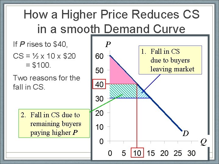
How a Higher Price Reduces CS in a smooth Demand Curve If P rises to $40, CS = ½ x 10 x $20 = $100. P 1. Fall in CS due to buyers leaving market Two reasons for the fall in CS. 2. Fall in CS due to remaining buyers paying higher P D Q

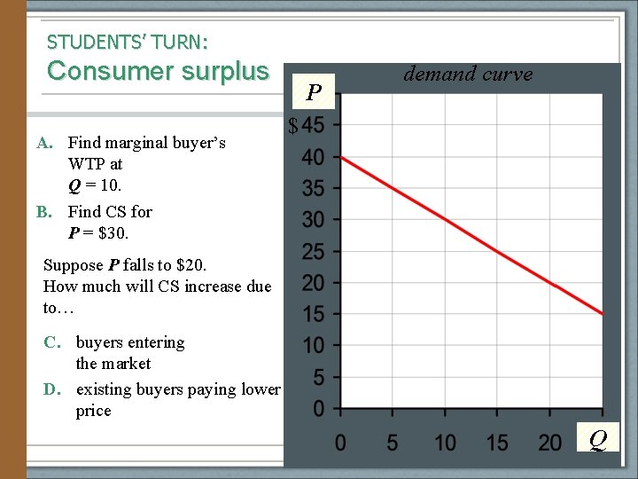
STUDENTS’ TURN: Consumer surplus A. Find marginal buyer’s WTP at Q = 10. B. Find CS for P = $30. P demand curve $ Suppose P falls to $20. How much will CS increase due to… C. buyers entering the market D. existing buyers paying lower price Q

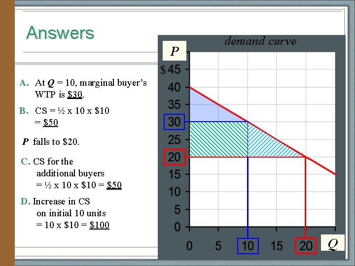
Answers P demand curve $ A. At Q = 10, marginal buyer’s WTP is $30. B. CS = ½ x 10 x $10 = $50 P falls to $20. C. CS for the additional buyers = ½ x 10 x $10 = $50 D. Increase in CS on initial 10 units = 10 x $10 = $100 Q

Principles of Microeconomics 09. Market Efficiency and Welfare* Juan Pablo Chauvin August 4, 2011 * Slide content principally sourced from N. Gregory Mankiw “Principles of Economics” Premium Powe. Point