Principles of Magnetic Resonance Imaging J Peter Mustonen

Principles of Magnetic Resonance Imaging J. Peter Mustonen (from David J. Michalak) Presentation for Physics 250 05/01/2008

Outline Ø Motivation Ø Principles of NMR Ø Interactions of spins in B 0 field Ø Principles of 1 D-MRI Ø Principles of 2 D-MRI Ø Summary

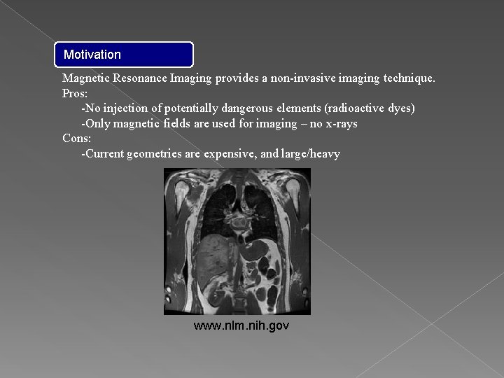
Motivation Magnetic Resonance Imaging provides a non-invasive imaging technique. Pros: -No injection of potentially dangerous elements (radioactive dyes) -Only magnetic fields are used for imaging – no x-rays Cons: -Current geometries are expensive, and large/heavy www. nlm. nih. gov

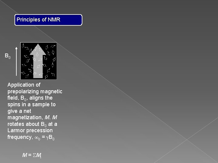
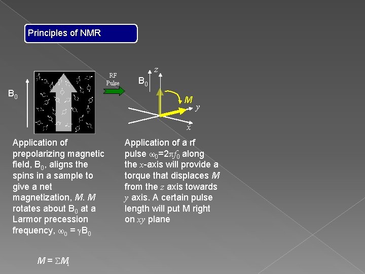
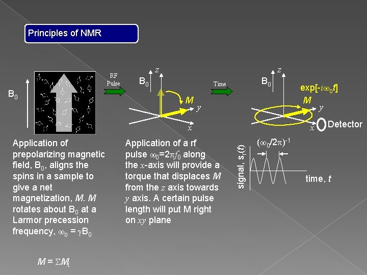
Principles of NMR B 0 Application of prepolarizing magnetic field, B 0, aligns the spins in a sample to give a net magnetization, M. M rotates about B 0 at a Larmor precession frequency, w 0 = g. B 0 M = SMi

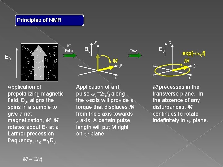
Principles of NMR RF Pulse B 0 z B 0 M y x Application of prepolarizing magnetic field, B 0, aligns the spins in a sample to give a net magnetization, M. M rotates about B 0 at a Larmor precession frequency, w 0 = g. B 0 M = SMi Application of a rf pulse w 0=2 pf 0 along the x-axis will provide a torque that displaces M from the z axis towards y axis. A certain pulse length will put M right on xy plane

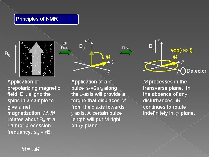
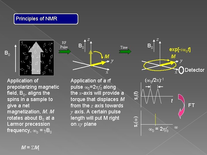
Principles of NMR RF Pulse B 0 z z B 0 Time M y x Application of prepolarizing magnetic field, B 0, aligns the spins in a sample to give a net magnetization, M. M rotates about B 0 at a Larmor precession frequency, w 0 = g. B 0 M = SMi Application of a rf pulse w 0=2 pf 0 along the x-axis will provide a torque that displaces M from the z axis towards y axis. A certain pulse length will put M right on xy plane B 0 exp[-iw 0 t] M y x M precesses in the transverse plane. In the absence of any disturbances, M continues to rotate indefinitely in xy plane.

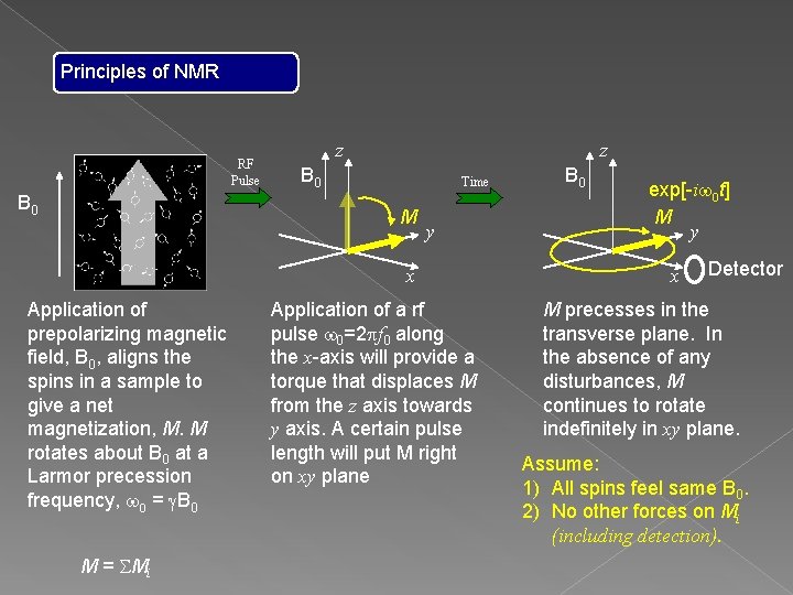
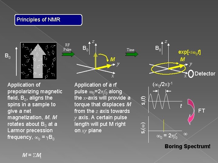
Principles of NMR RF Pulse B 0 z z B 0 Time M y x Application of prepolarizing magnetic field, B 0, aligns the spins in a sample to give a net magnetization, M. M rotates about B 0 at a Larmor precession frequency, w 0 = g. B 0 M = SMi Application of a rf pulse w 0=2 pf 0 along the x-axis will provide a torque that displaces M from the z axis towards y axis. A certain pulse length will put M right on xy plane B 0 exp[-iw 0 t] M y x Detector M precesses in the transverse plane. In the absence of any disturbances, M continues to rotate indefinitely in xy plane.

Principles of NMR RF Pulse B 0 z z B 0 Time M y x Application of prepolarizing magnetic field, B 0, aligns the spins in a sample to give a net magnetization, M. M rotates about B 0 at a Larmor precession frequency, w 0 = g. B 0 M = SMi Application of a rf pulse w 0=2 pf 0 along the x-axis will provide a torque that displaces M from the z axis towards y axis. A certain pulse length will put M right on xy plane B 0 exp[-iw 0 t] M y x Detector M precesses in the transverse plane. In the absence of any disturbances, M continues to rotate indefinitely in xy plane. Assume: 1) All spins feel same B 0. 2) No other forces on Mi (including detection).

Principles of NMR RF Pulse B 0 z z B 0 Time M y Application of prepolarizing magnetic field, B 0, aligns the spins in a sample to give a net magnetization, M. M rotates about B 0 at a Larmor precession frequency, w 0 = g. B 0 M = SMi Application of a rf pulse w 0=2 pf 0 along the x-axis will provide a torque that displaces M from the z axis towards y axis. A certain pulse length will put M right on xy plane x signal, sr(t) x exp[-iw 0 t] M y Detector (w 0/2 p)-1 time, t

Principles of NMR RF Pulse B 0 z z B 0 Time M y exp[-iw 0 t] M y x M = SMi Detector (w 0/2 p)-1 sr(t) Application of a rf pulse w 0=2 pf 0 along the x-axis will provide a torque that displaces M from the z axis towards y axis. A certain pulse length will put M right on xy plane sr(w) Application of prepolarizing magnetic field, B 0, aligns the spins in a sample to give a net magnetization, M. M rotates about B 0 at a Larmor precession frequency, w 0 = g. B 0 x t w 0 = 2 pf 0 FT w

Principles of NMR RF Pulse B 0 z z B 0 Time M exp[-iw 0 t] M y y x Detector (w 0/2 p)-1 sr(t) Application of a rf pulse w 0=2 pf 0 along the x-axis will provide a torque that displaces M from the z axis towards y axis. A certain pulse length will put M right on xy plane sr(w) Application of prepolarizing magnetic field, B 0, aligns the spins in a sample to give a net magnetization, M. M rotates about B 0 at a Larmor precession frequency, w 0 = g. B 0 x t w 0 = 2 pf 0 FT w Boring Spectrum! M = SMi

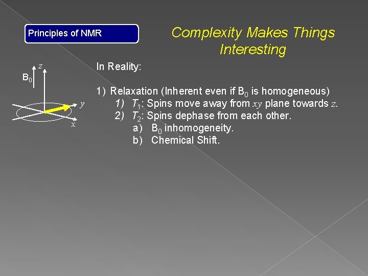
Principles of NMR z Complexity Makes Things Interesting In Reality: B 0 y x 1) Relaxation (Inherent even if B 0 is homogeneous) 1) T 1: Spins move away from xy plane towards z. 2) T 2: Spins dephase from each other. a) B 0 inhomogeneity. b) Chemical Shift.

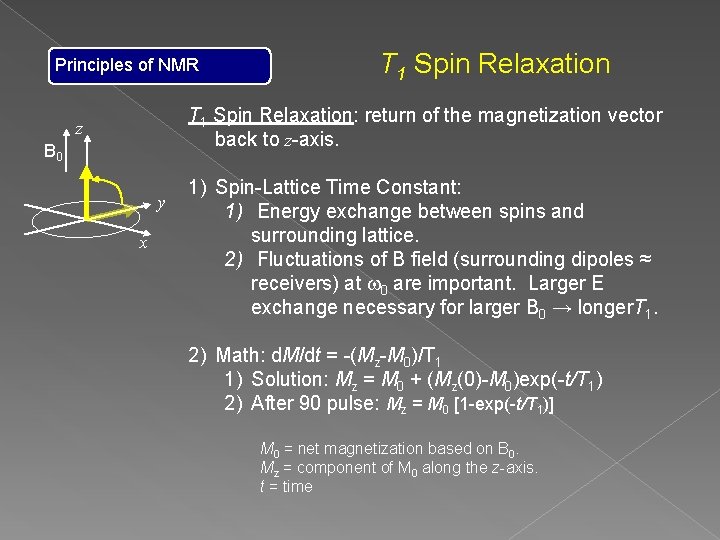
Principles of NMR T 1 Spin Relaxation: return of the magnetization vector back to z-axis. z B 0 y x 1) Spin-Lattice Time Constant: 1) Energy exchange between spins and surrounding lattice. 2) Fluctuations of B field (surrounding dipoles ≈ receivers) at w 0 are important. Larger E exchange necessary for larger B 0 → longer. T 1. 2) Math: d. M/dt = -(Mz-M 0)/T 1 1) Solution: Mz = M 0 + (Mz(0)-M 0)exp(-t/T 1) 2) After 90 pulse: Mz = M 0 [1 -exp(-t/T 1)] M 0 = net magnetization based on B 0. Mz = component of M 0 along the z-axis. t = time

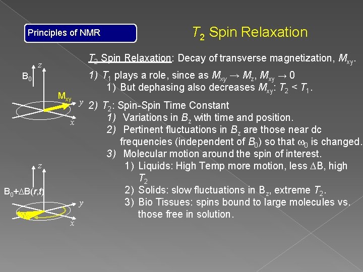
Principles of NMR T 2 Spin Relaxation: Decay of transverse magnetization, Mxy. z 1) T 1 plays a role, since as Mxy → Mz, Mxy → 0 1) But dephasing also decreases Mxy: T 2 < T 1. B 0 Mxy y 2) T : Spin-Spin Time Constant 2 x z B 0+DB(r, t) y x 1) Variations in Bz with time and position. 2) Pertinent fluctuations in Bz are those near dc frequencies (independent of B 0) so that w 0 is changed. 3) Molecular motion around the spin of interest. 1) Liquids: High Temp more motion, less DB, high T 2 2) Solids: slow fluctuations in Bz, extreme T 2. 3) Bio Tissues: spins bound to large molecules vs. those free in solution.

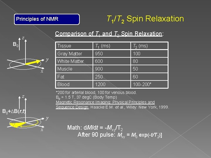
T 1/T 2 Spin Relaxation Principles of NMR Comparison of T 1 and T 2 Spin Relaxation: z B 0 y x Tissue T 1 (ms) T 2 (ms) Gray Matter 950 100 White Matter 600 80 Muscle 900 50 Fat 250 60 Blood 1200 100 -200* *200 for arterial blood, 100 for venous blood. B 0 = 1. 5 T, 37 deg. C (Body Temp) Magnetic Resonance Imaging: Physical Principles and Sequence Design, Haacke E. M. et al. , Wiley: New York, 1999. z B 0+DB(r, t) y x Math: d. M/dt = -Mxy/T 2 After 90 pulse: Mxy = M 0 exp(-t/T 2)]

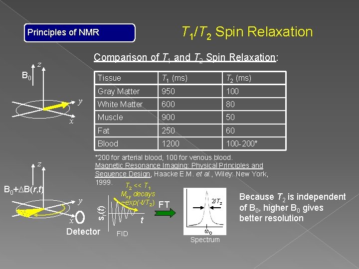
T 1/T 2 Spin Relaxation Principles of NMR Comparison of T 1 and T 2 Spin Relaxation: z B 0 y x T 1 (ms) T 2 (ms) Gray Matter 950 100 White Matter 600 80 Muscle 900 50 Fat 250 60 Blood 1200 100 -200* *200 for arterial blood, 100 for venous blood. Magnetic Resonance Imaging: Physical Principles and Sequence Design, Haacke E. M. et al. , Wiley: New York, 1999. T << T z 2 y sr(t) B 0+DB(r, t) Tissue x Detector 1 Mxy decays ~exp(-t/T 2) FT 2/T 2 t FID w 0 Spectrum Because T 2 is independent of B 0, higher B 0 gives better resolution

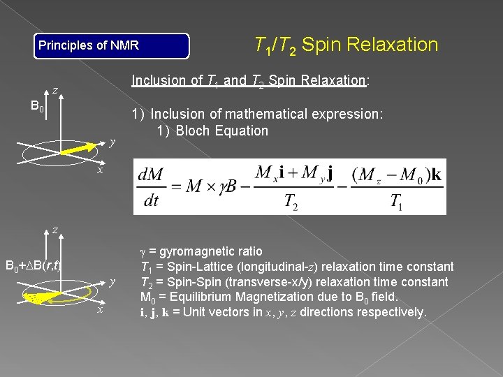
Principles of NMR T 1/T 2 Spin Relaxation Inclusion of T 1 and T 2 Spin Relaxation: z B 0 y 1) Inclusion of mathematical expression: 1) Bloch Equation x z B 0+DB(r, t) y x g = gyromagnetic ratio T 1 = Spin-Lattice (longitudinal-z) relaxation time constant T 2 = Spin-Spin (transverse-x/y) relaxation time constant M 0 = Equilibrium Magnetization due to B 0 field. i, j, k = Unit vectors in x, y, z directions respectively.

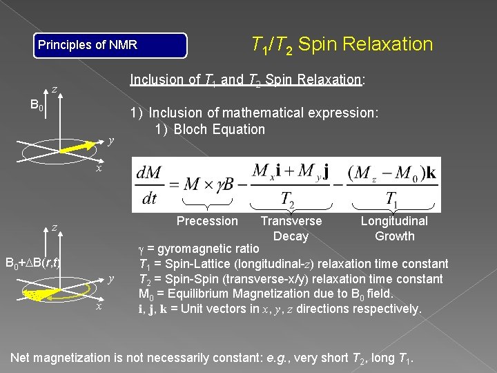
T 1/T 2 Spin Relaxation Principles of NMR Inclusion of T 1 and T 2 Spin Relaxation: z B 0 y 1) Inclusion of mathematical expression: 1) Bloch Equation x Precession z B 0+DB(r, t) y x Transverse Decay Longitudinal Growth g = gyromagnetic ratio T 1 = Spin-Lattice (longitudinal-z) relaxation time constant T 2 = Spin-Spin (transverse-x/y) relaxation time constant M 0 = Equilibrium Magnetization due to B 0 field. i, j, k = Unit vectors in x, y, z directions respectively. Net magnetization is not necessarily constant: e. g. , very short T 2, long T 1.

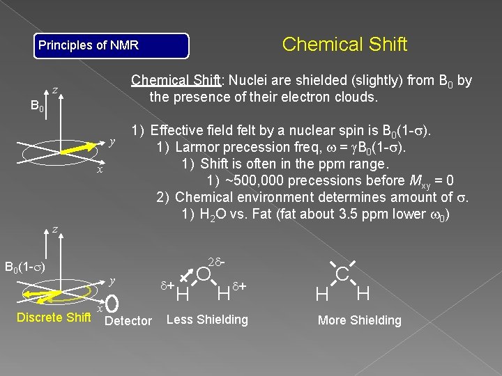
Chemical Shift Principles of NMR Chemical Shift: Nuclei are shielded (slightly) from B 0 by the presence of their electron clouds. z B 0 y x z 2 d- B 0(1 -s) Discrete Shift 1) Effective field felt by a nuclear spin is B 0(1 -s). 1) Larmor precession freq, w = g. B 0(1 -s). 1) Shift is often in the ppm range. 1) ~500, 000 precessions before Mxy = 0 2) Chemical environment determines amount of s. 1) H 2 O vs. Fat (fat about 3. 5 ppm lower w 0) y x Detector d+ H O H d+ Less Shielding H C H More Shielding

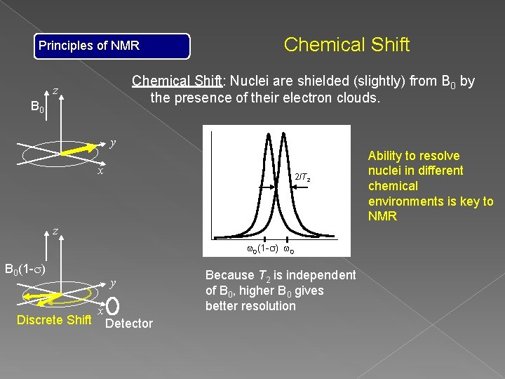
Principles of NMR Chemical Shift: Nuclei are shielded (slightly) from B 0 by the presence of their electron clouds. z B 0 y x 2/T 2 z w 0(1 -s) w 0 B 0(1 -s) Discrete Shift y x Detector Because T 2 is independent of B 0, higher B 0 gives better resolution Ability to resolve nuclei in different chemical environments is key to NMR

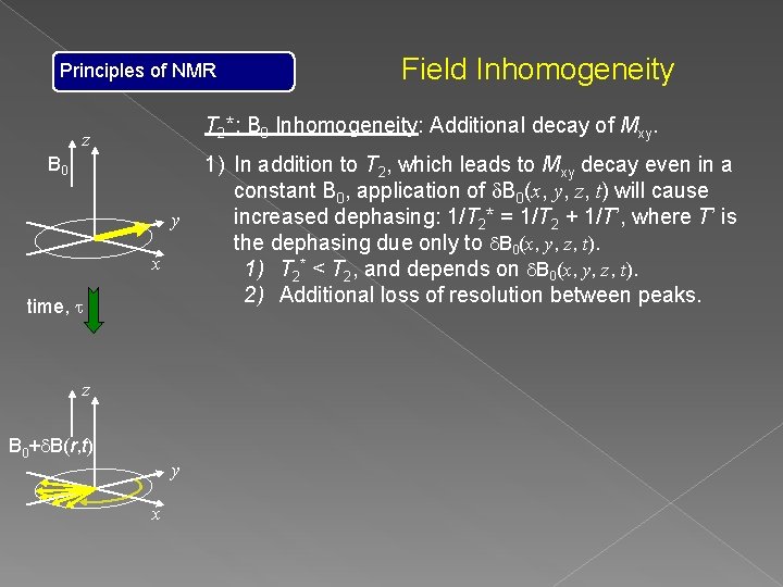
Principles of NMR Field Inhomogeneity T 2*: B 0 Inhomogeneity: Additional decay of Mxy. z B 0 y x time, t z B 0+d. B(r, t) y x 1) In addition to T 2, which leads to Mxy decay even in a constant B 0, application of d. B 0(x, y, z, t) will cause increased dephasing: 1/T 2* = 1/T 2 + 1/T’, where T’ is the dephasing due only to d. B 0(x, y, z, t). 1) T 2* < T 2, and depends on d. B 0(x, y, z, t). 2) Additional loss of resolution between peaks.

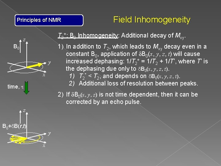
Principles of NMR Field Inhomogeneity T 2*: B 0 Inhomogeneity: Additional decay of Mxy. z B 0 y x time, t 1) In addition to T 2, which leads to Mxy decay even in a constant B 0, application of d. B 0(x, y, z, t) will cause increased dephasing: 1/T 2* = 1/T 2 + 1/T’, where T’ is the dephasing due only to d. B 0(x, y, z, t). 1) T 2* < T 2, and depends on d. B 0(x, y, z, t). 2) Additional loss of resolution between peaks. 2) If d. B 0(x, y, z) is not time dependent, then it can be corrected by an echo pulse. z B 0+d. B(r, t) y x

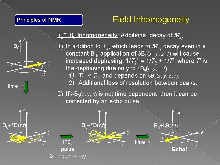
Field Inhomogeneity Principles of NMR T 2*: B 0 Inhomogeneity: Additional decay of Mxy. z B 0 y x time, t 1) In addition to T 2, which leads to Mxy decay even in a constant B 0, application of d. B 0(x, y, z, t) will cause increased dephasing: 1/T 2* = 1/T 2 + 1/T’, where T’ is the dephasing due only to d. B 0(x, y, z, t). 1) T 2* < T 2, and depends on d. B 0(x, y, z, t). 2) Additional loss of resolution between peaks. 2) If d. B 0(x, y, z) is not time dependent, then it can be corrected by an echo pulse. z z z B 0+d. B(r, t) y x 180 x pulse (x → x, y → –y) y x time, t Echo! y x

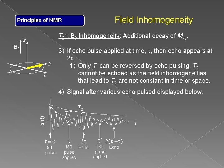
Field Inhomogeneity Principles of NMR T 2*: B 0 Inhomogeneity: Additional decay of Mxy. z B 0 y x 3) If echo pulse applied at time, t, then echo appears at 2 t. 1) Only T’ can be reversed by echo pulsing, T 2 cannot be echoed as the field inhomogeneities that lead to T 2 are not constant in time or space. sr(t) 4) Signal after various echo pulsed displayed below. t=0 90 pulse T 2 * T 2 t t 2 t 180 Echo pulse applied t’ 2(t’-t) 180 Echo pulse applied

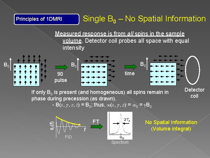
Single B 0 – No Spatial Information Principles of 1 DMRI Measured response is from all spins in the sample volume. Detector coil probes all space with equal intensity B 0 B 0 time 90 pulse If only B 0 is present (and homogeneous) all spins remain in phase during precession (as drawn). - B(x, y, z, t) = B 0; thus, w(x, y, z) = w 0 = g. B 0 sr(t) FT 2/T 2 t FID w 0 Spectrum Detector coil No Spatial Information (Volume integral)

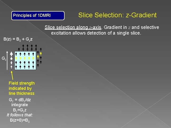
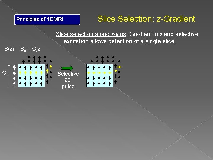
Principles of 1 DMRI Slice Selection: z-Gradient Slice selection along z-axis. Gradient in z and selective excitation allows detection of a single slice. B(z) = B 0 + Gzz Gz Field strength indicated by line thickness Gz = d. Bz/dz integrate Bz=Gzz It follows that: B(z=0)=B 0

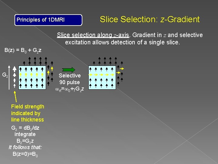
Principles of 1 DMRI Slice Selection: z-Gradient Slice selection along z-axis. Gradient in z and selective excitation allows detection of a single slice. B(z) = B 0 + Gzz Gz Selective 90 pulse wrf=w 0+g. Gzz Field strength indicated by line thickness Gz = d. Bz/dz integrate Bz=Gzz It follows that: B(z=0)=B 0

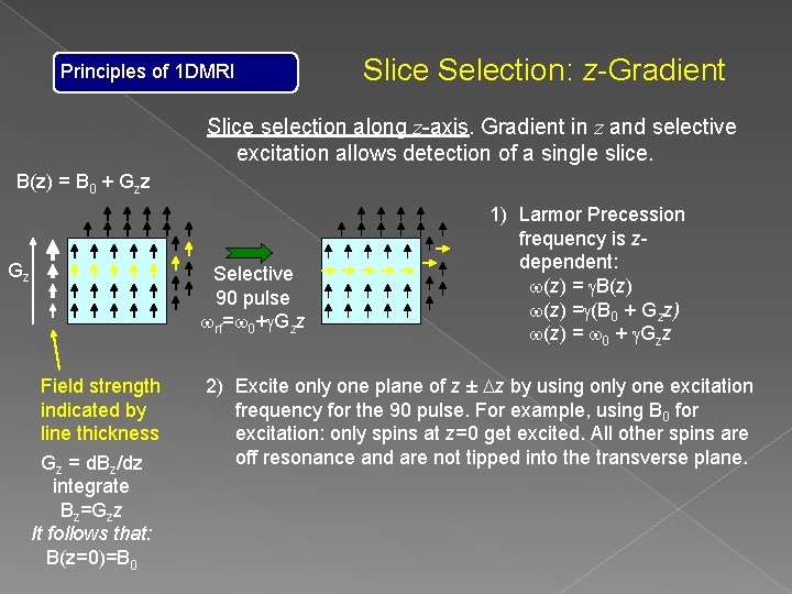
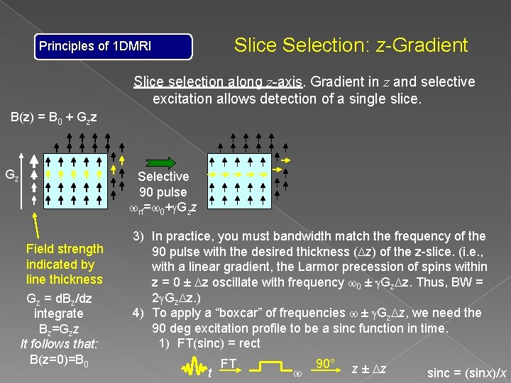
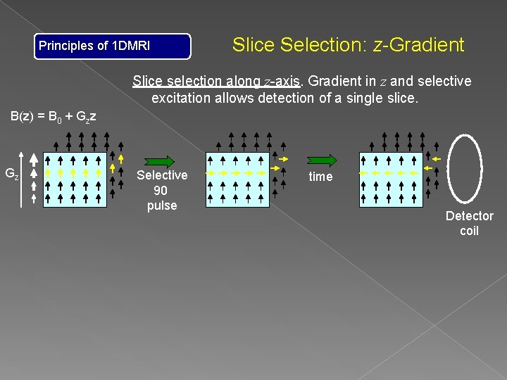
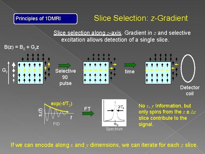
Principles of 1 DMRI Slice Selection: z-Gradient Slice selection along z-axis. Gradient in z and selective excitation allows detection of a single slice. B(z) = B 0 + Gzz Gz Selective 90 pulse wrf=w 0+g. Gzz Field strength indicated by line thickness Gz = d. Bz/dz integrate Bz=Gzz It follows that: B(z=0)=B 0 1) Larmor Precession frequency is zdependent: w(z) = g. B(z) w(z) =g(B 0 + Gzz) w(z) = w 0 + g. Gzz 2) Excite only one plane of z ± Dz by using only one excitation frequency for the 90 pulse. For example, using B 0 for excitation: only spins at z=0 get excited. All other spins are off resonance and are not tipped into the transverse plane.

Slice Selection: z-Gradient Principles of 1 DMRI Slice selection along z-axis. Gradient in z and selective excitation allows detection of a single slice. B(z) = B 0 + Gzz Gz Selective 90 pulse wrf=w 0+g. Gzz Field strength indicated by line thickness Gz = d. Bz/dz integrate Bz=Gzz It follows that: B(z=0)=B 0 3) In practice, you must bandwidth match the frequency of the 90 pulse with the desired thickness (Dz) of the z-slice. (i. e. , with a linear gradient, the Larmor precession of spins within z = 0 ± Dz oscillate with frequency w 0 ± g. Gz. Dz. Thus, BW = 2 g. Gz. Dz. ) 4) To apply a “boxcar” of frequencies w ± g. Gz. Dz, we need the 90 deg excitation profile to be a sinc function in time. 1) FT(sinc) = rect t FT w 90° z ± Dz sinc = (sinx)/x

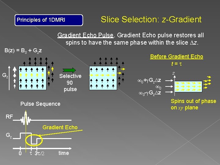
Principles of 1 DMRI Slice Selection: z-Gradient Echo Pulse. Gradient Echo pulse restores all spins to have the same phase within the slice Dz. B(z) = B 0 + Gzz Before Gradient Echo t=t Gz Selective 90 pulse Pulse Sequence RF Gradient Echo Gz 0 t 3 t/2 time z w 0+g. Gz. Dz w 0 -g. Gz. Dz Spins out of phase on xy plane

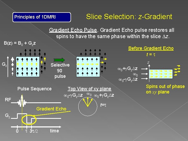
Slice Selection: z-Gradient Principles of 1 DMRI Gradient Echo Pulse. Gradient Echo pulse restores all spins to have the same phase within the slice Dz. B(z) = B 0 + Gzz Before Gradient Echo t=t Gz z Selective 90 pulse Pulse Sequence RF Top View of xy plane w 0 -g. Gz. Dz w 0+g. Gz. Dz Gradient Echo Gz 0 t 3 t/2 time w 0+g. Gz. Dz w 0 -g. Gz. Dz t=t Spins out of phase on xy plane

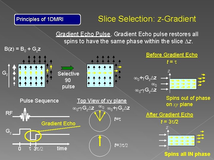
Slice Selection: z-Gradient Principles of 1 DMRI Gradient Echo Pulse. Gradient Echo pulse restores all spins to have the same phase within the slice Dz. B(z) = B 0 + Gzz Before Gradient Echo t=t Gz z Selective 90 pulse Pulse Sequence RF w 0+g. Gz. Dz w 0 -g. Gz. Dz Top View of xy plane w 0 -g. Gz. Dz w 0+g. Gz. Dz Gradient Echo t=t Gz 0 t 3 t/2 time Spins out of phase on xy plane After Gradient Echo t = 3 t/2 z t=3 t/2 Spins all IN phase

Principles of 1 DMRI Slice Selection: z-Gradient Slice selection along z-axis. Gradient in z and selective excitation allows detection of a single slice. B(z) = B 0 + Gzz Gz Selective 90 pulse

Principles of 1 DMRI Slice Selection: z-Gradient Slice selection along z-axis. Gradient in z and selective excitation allows detection of a single slice. B(z) = B 0 + Gzz Gz Selective 90 pulse time Detector coil

Slice Selection: z-Gradient Principles of 1 DMRI Slice selection along z-axis. Gradient in z and selective excitation allows detection of a single slice. B(z) = B 0 + Gzz Gz Selective 90 pulse sr(t) exp(-t/T 2) time Detector coil FT 2/T 2 t FID w 0 Spectrum No x, y Information, but only spins from the z ± Dz slice contribute to the signal. If we can encode along x and y dimensions, we can iterate for each z slice.

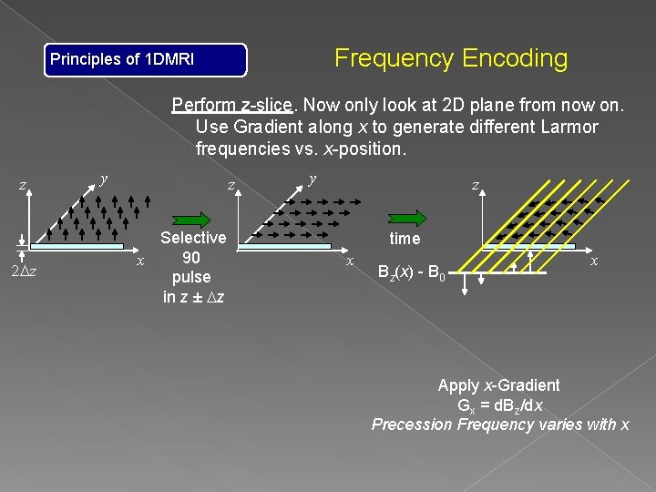
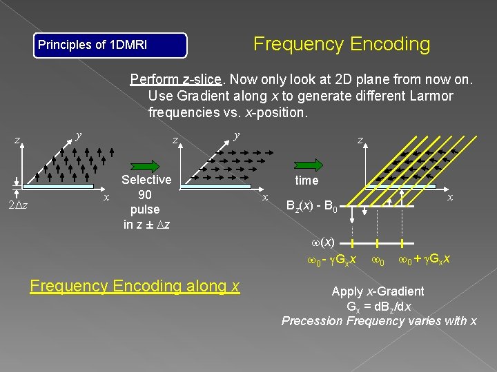
Frequency Encoding Principles of 1 DMRI Perform z-slice. Now only look at 2 D plane from now on. Use Gradient along x to generate different Larmor frequencies vs. x-position. z 2 Dz y z Selective 90 x pulse in z ± Dz y z time x Bz(x) - B 0 x Apply x-Gradient Gx = d. Bz/dx Precession Frequency varies with x

Frequency Encoding Principles of 1 DMRI Perform z-slice. Now only look at 2 D plane from now on. Use Gradient along x to generate different Larmor frequencies vs. x-position. z 2 Dz y Selective 90 x pulse in z ± Dz z time x Bz(x) - B 0 w(x) w 0 - g. Gxx Frequency Encoding along x x w 0 + g. Gxx Apply x-Gradient Gx = d. Bz/dx Precession Frequency varies with x

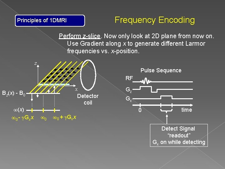
Frequency Encoding Principles of 1 DMRI Perform z-slice. Now only look at 2 D plane from now on. Use Gradient along x to generate different Larmor frequencies vs. x-position. z Pulse Sequence RF x Detector coil Bz(x) - B 0 w(x) w 0 - g. Gxx w 0 + g. Gxx Gz Gx 0 time Detect Signal “readout” Gx on while detecting

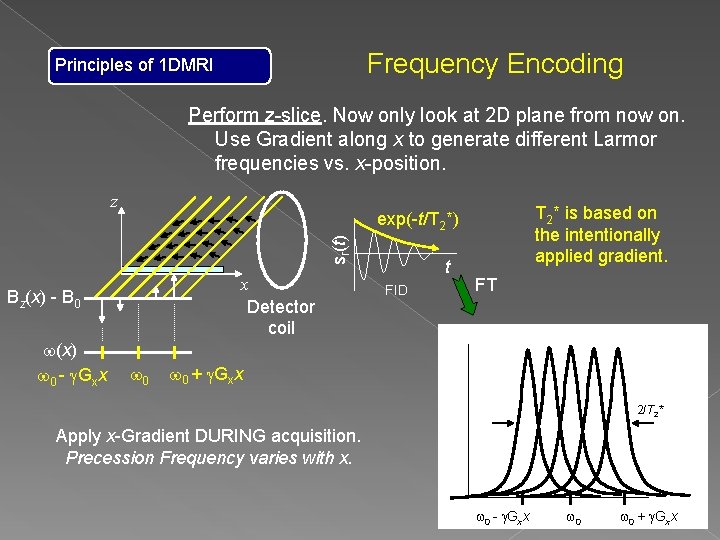
Frequency Encoding Principles of 1 DMRI Perform z-slice. Now only look at 2 D plane from now on. Use Gradient along x to generate different Larmor frequencies vs. x-position. z sr(t) x Detector coil Bz(x) - B 0 w(x) w 0 - g. Gxx T 2* is based on the intentionally applied gradient. exp(-t/T 2*) w 0 t FID FT w 0 + g. Gxx 2/T 2* Apply x-Gradient DURING acquisition. Precession Frequency varies with x. w 0 - g. Gxx w 0 + g. Gxx

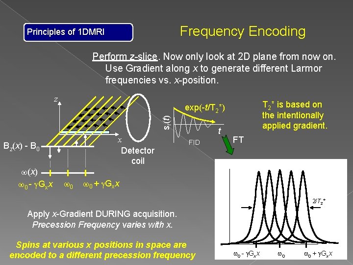
Frequency Encoding Principles of 1 DMRI Perform z-slice. Now only look at 2 D plane from now on. Use Gradient along x to generate different Larmor frequencies vs. x-position. z sr(t) x Detector coil Bz(x) - B 0 w(x) w 0 - g. Gxx T 2* is based on the intentionally applied gradient. exp(-t/T 2*) w 0 t FID FT w 0 + g. Gxx 2/T 2* Apply x-Gradient DURING acquisition. Precession Frequency varies with x. Spins at various x positions in space are encoded to a different precession frequency w 0 - g. Gxx w 0 + g. Gxx

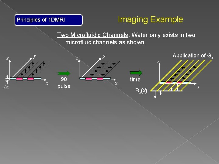
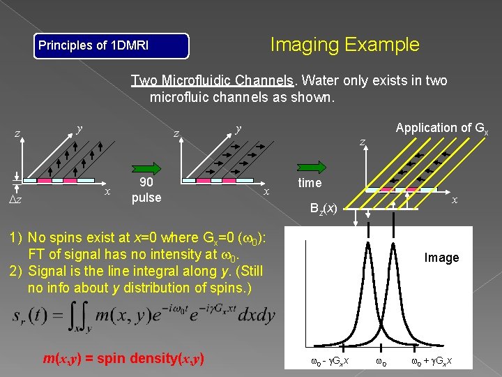
Imaging Example Principles of 1 DMRI Two Microfluidic Channels. Water only exists in two microfluic channels as shown. z Dz y z x 90 pulse y z x Application of Gx time Bz(x) x

Imaging Example Principles of 1 DMRI Two Microfluidic Channels. Water only exists in two microfluic channels as shown. z Dz y z x 90 pulse y Application of Gx z x time x Bz(x) 1) No spins exist at x=0 where Gx=0 (w 0): FT of signal has no intensity at w 0. 2) Signal is the line integral along y. (Still no info about y distribution of spins. ) m(x, y) = spin density(x, y) Image w 0 - g. Gxx w 0 + g. Gxx

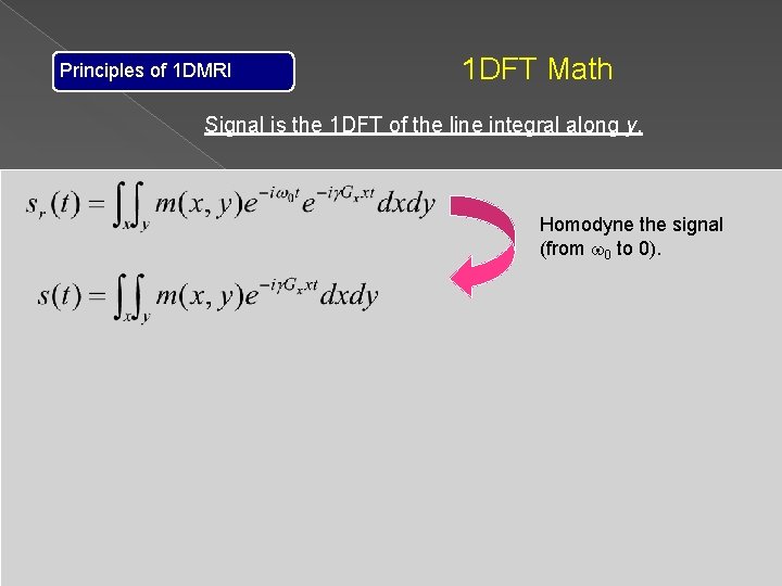
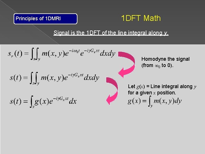
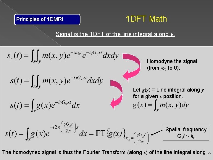
Principles of 1 DMRI 1 DFT Math Signal is the 1 DFT of the line integral along y. Homodyne the signal (from w 0 to 0).

Principles of 1 DMRI 1 DFT Math Signal is the 1 DFT of the line integral along y. Homodyne the signal (from w 0 to 0). Let g(x) = Line integral along y for a given x position.

Principles of 1 DMRI 1 DFT Math Signal is the 1 DFT of the line integral along y. Homodyne the signal (from w 0 to 0). Let g(x) = Line integral along y for a given x position. Spatial frequency Gxt ~ kx The homodyned signal is thus the Fourier Transform (along x) of the line integral along y.

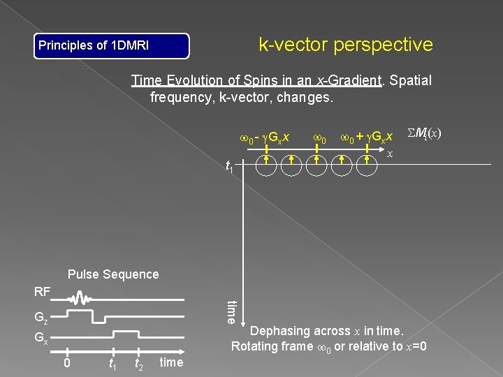
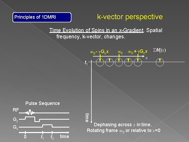
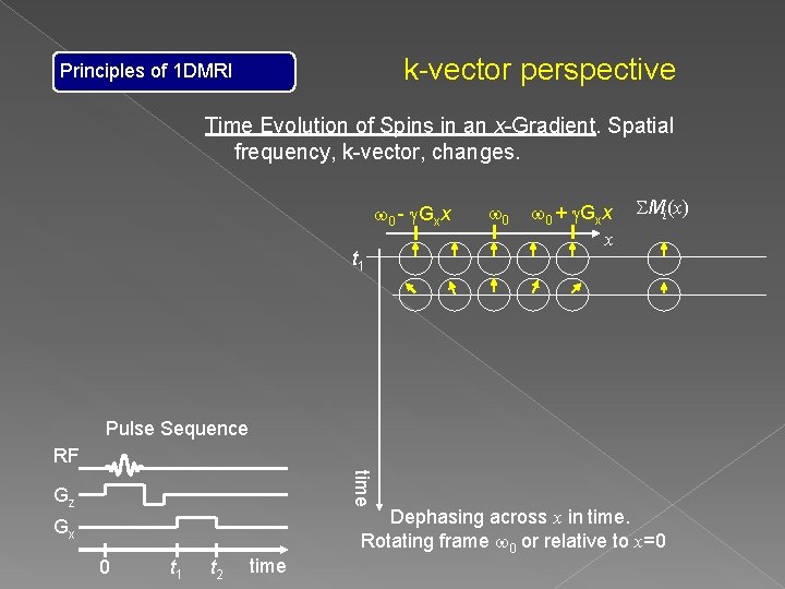
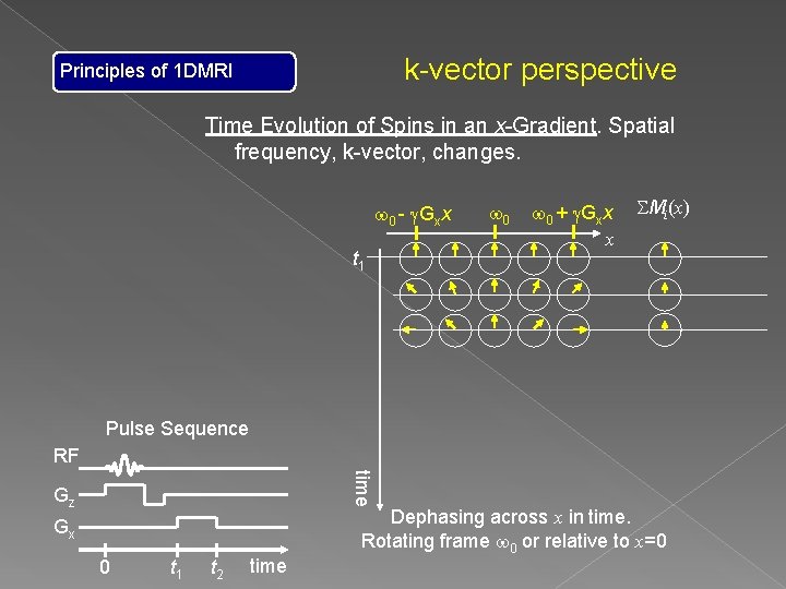
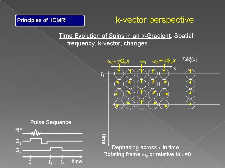
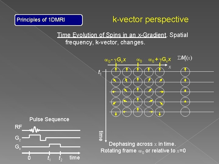
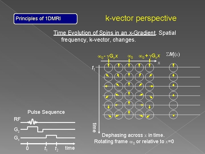
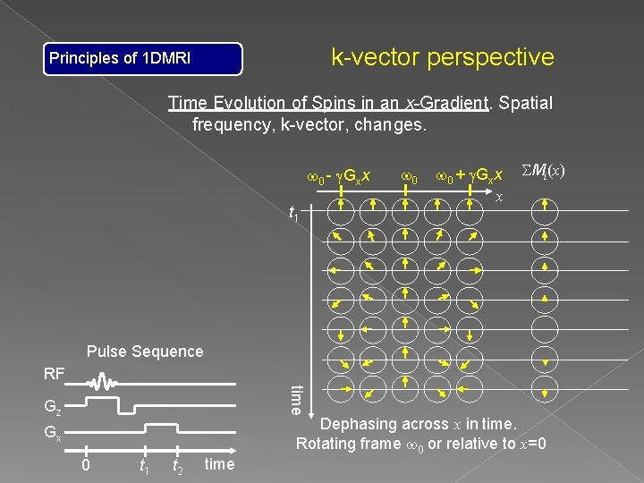
k-vector perspective Principles of 1 DMRI Time Evolution of Spins in an x-Gradient. Spatial frequency, k-vector, changes. w 0 - g. Gxx t 1 w 0 + g. Gxx x SMi(x) Pulse Sequence RF time Gz Gx 0 t 1 t 2 time Dephasing across x in time. Rotating frame w 0 or relative to x=0

k-vector perspective Principles of 1 DMRI Time Evolution of Spins in an x-Gradient. Spatial frequency, k-vector, changes. w 0 - g. Gxx t 1 w 0 + g. Gxx x SMi(x) Pulse Sequence RF time Gz Gx 0 t 1 t 2 time Dephasing across x in time. Rotating frame w 0 or relative to x=0

k-vector perspective Principles of 1 DMRI Time Evolution of Spins in an x-Gradient. Spatial frequency, k-vector, changes. w 0 - g. Gxx t 1 w 0 + g. Gxx x SMi(x) Pulse Sequence RF time Gz Gx 0 t 1 t 2 time Dephasing across x in time. Rotating frame w 0 or relative to x=0

k-vector perspective Principles of 1 DMRI Time Evolution of Spins in an x-Gradient. Spatial frequency, k-vector, changes. w 0 - g. Gxx t 1 w 0 + g. Gxx x SMi(x) Pulse Sequence RF time Gz Gx 0 t 1 t 2 time Dephasing across x in time. Rotating frame w 0 or relative to x=0

k-vector perspective Principles of 1 DMRI Time Evolution of Spins in an x-Gradient. Spatial frequency, k-vector, changes. w 0 - g. Gxx t 1 w 0 + g. Gxx x SMi(x) Pulse Sequence RF time Gz Gx 0 t 1 t 2 time Dephasing across x in time. Rotating frame w 0 or relative to x=0

k-vector perspective Principles of 1 DMRI Time Evolution of Spins in an x-Gradient. Spatial frequency, k-vector, changes. w 0 - g. Gxx t 1 w 0 + g. Gxx x SMi(x) Pulse Sequence RF time Gz Gx 0 t 1 t 2 time Dephasing across x in time. Rotating frame w 0 or relative to x=0

k-vector perspective Principles of 1 DMRI Time Evolution of Spins in an x-Gradient. Spatial frequency, k-vector, changes. w 0 - g. Gxx t 1 w 0 + g. Gxx x SMi(x) Pulse Sequence RF time Gz Gx 0 t 1 t 2 time Dephasing across x in time. Rotating frame w 0 or relative to x=0

k-vector perspective Principles of 1 DMRI Time Evolution of Spins in an x-Gradient. Spatial frequency, k-vector, changes. w 0 - g. Gxx t 1 w 0 + g. Gxx x SMi(x) Pulse Sequence RF time Gz Gx 0 t 1 t 2 time Dephasing across x in time. Rotating frame w 0 or relative to x=0

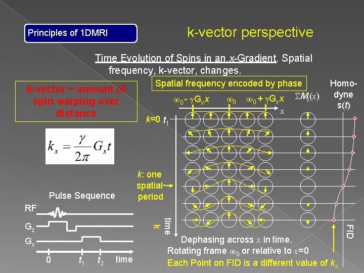
k-vector perspective Principles of 1 DMRI Time Evolution of Spins in an x-Gradient. Spatial frequency, k-vector, changes. k-vector ~ amount of spin warping over distance Spatial frequency encoded by phase w + g. G x SMi(x) w w - g. G x 0 k=0 t 1 x 0 0 x x Homodyne s(t) k: one spatial period Pulse Sequence RF Gx 0 t 1 t 2 time Dephasing across x in time. Rotating frame w 0 or relative to x=0 Each Point on FID is a different value of kx FID time k Gz

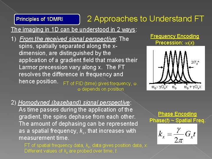
Principles of 1 DMRI 2 Approaches to Understand FT The imaging in 1 D can be understood in 2 ways: 1) From the received signal perspective: The spins, spatially separated along the xdimension, are distinguished by the application of a gradient field that makes their Larmor precession vary along x. The FT resolves the difference in frequency and hence position. FT of FID (time) gives frequency, w. w depends on position 2) Homodyned (baseband) signal perspective: As time passes during the application of the gradient, the spins dephase from each other. The amount of dephasing can be represented as a spatial frequency, kx, that increases with measurement time. FT of spatial frequency data, kx, data gives position data, x. Different values of kx are probed over time, t. Frequency Encoding Precession: w(x) 2/T 2* w 0 - g. Gxx w 0 + g. Gxx Phase Encoding Phase(t) ~ Spatial Freq.

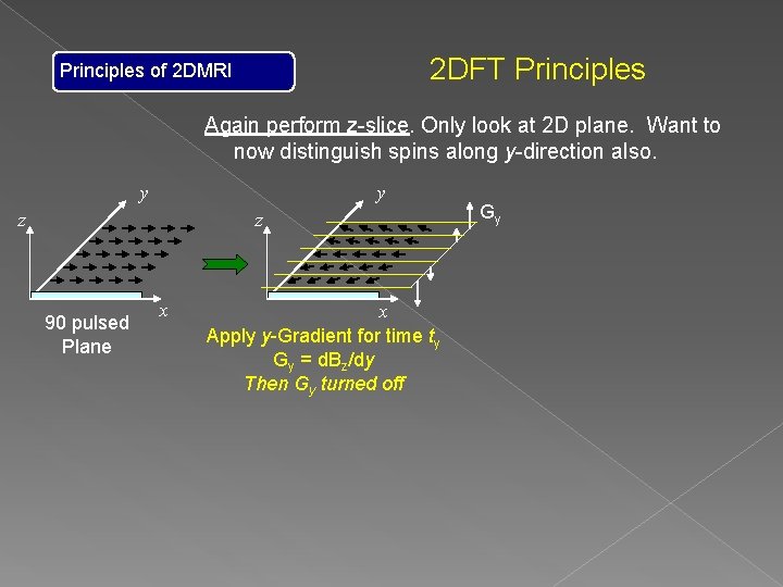
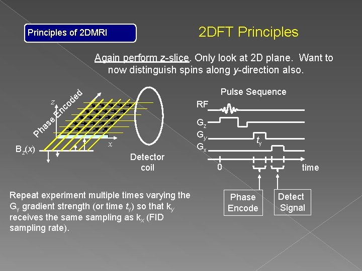
2 DFT Principles of 2 DMRI Again perform z-slice. Only look at 2 D plane. Want to now distinguish spins along y-direction also. y y z z 90 pulsed Plane x x Apply y-Gradient for time ty Gy = d. Bz/dy Then Gy turned off Gy

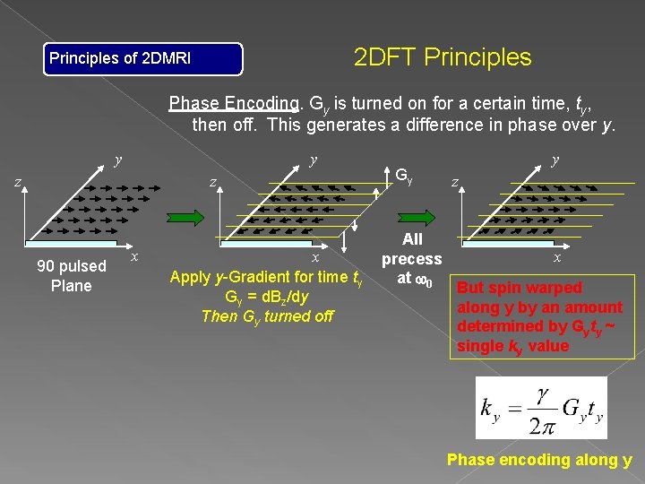
2 DFT Principles of 2 DMRI Phase Encoding. Gy is turned on for a certain time, ty, then off. This generates a difference in phase over y. y y z z 90 pulsed Plane x x Apply y-Gradient for time ty Gy = d. Bz/dy Then Gy turned off Gy All precess at w 0 y z x But spin warped along y by an amount determined by Gyty ~ single ky value Phase encoding along y

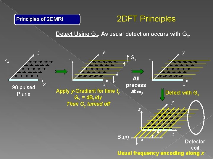
2 DFT Principles of 2 DMRI Detect Using Gx. As usual detection occurs with Gx. y y z Gy z 90 pulsed Plane x y x Apply y-Gradient for time ty Gy = d. Bz/dy Then Gy turned off z All precess at w 0 Bz(x) x Detect with Gx y z x Detector coil Usual frequency encoding along x

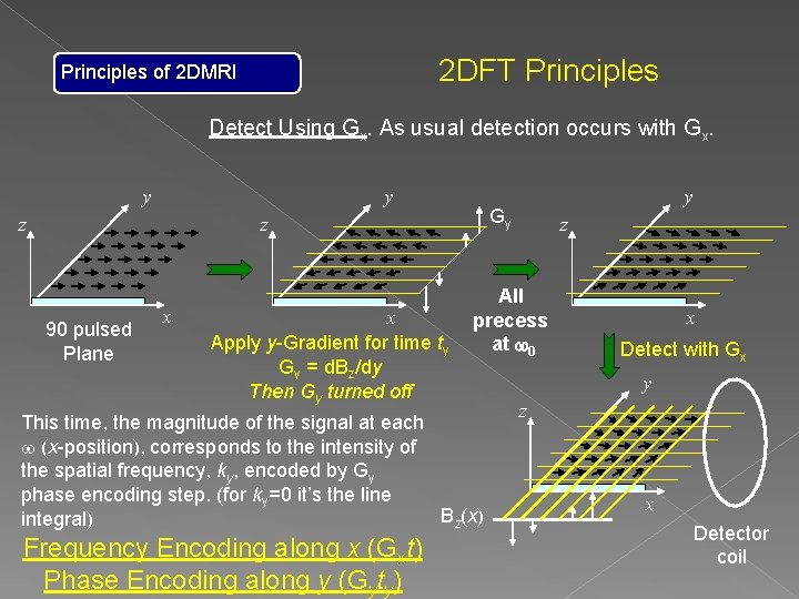
2 DFT Principles of 2 DMRI Detect Using Gx. As usual detection occurs with Gx. y y z Gy z 90 pulsed Plane x x Apply y-Gradient for time ty Gy = d. Bz/dy Then Gy turned off z All precess at w 0 This time, the magnitude of the signal at each w (x-position), corresponds to the intensity of the spatial frequency, ky, encoded by Gy phase encoding step. (for ky=0 it’s the line Bz(x) integral) Frequency Encoding along x (Gxt) Phase Encoding along y (Gyty) y x Detect with Gx y z x Detector coil

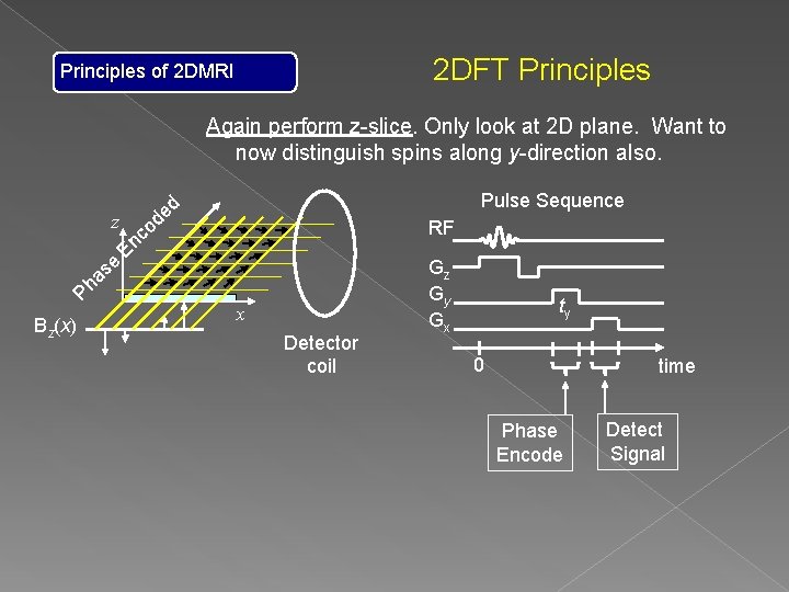
2 DFT Principles of 2 DMRI Again perform z-slice. Only look at 2 D plane. Want to now distinguish spins along y-direction also. z e s ha P Bz(x) Pulse Sequence d de o c En RF x Detector coil Gz Gy Gx ty 0 time Phase Encode Detect Signal

2 DFT Principles of 2 DMRI Again perform z-slice. Only look at 2 D plane. Want to now distinguish spins along y-direction also. z e s ha P Bz(x) Pulse Sequence d de o c En RF x Detector coil Repeat experiment multiple times varying the Gy gradient strength (or time ty) so that ky receives the sampling as kx (FID sampling rate). Gz Gy Gx ty 0 time Phase Encode Detect Signal

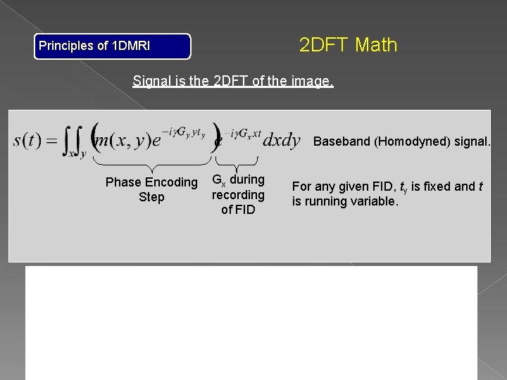
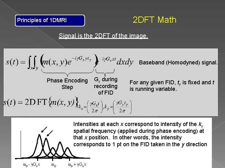
2 DFT Math Principles of 1 DMRI Signal is the 2 DFT of the image. Baseband (Homodyned) signal. Phase Encoding Step Gx during recording of FID For any given FID, ty is fixed and t is running variable.

2 DFT Math Principles of 1 DMRI Signal is the 2 DFT of the image. Baseband (Homodyned) signal. Phase Encoding Step Gx during recording of FID For any given FID, ty is fixed and t is running variable. Intensities at each x correspond to intensity of the ky spatial frequency (applied during phase encoding) at that x position. In other words, the intensity corresponds to 1 pt on the FID taken in the y direction w 0 - g. Gxx w 0 + g. Gxx

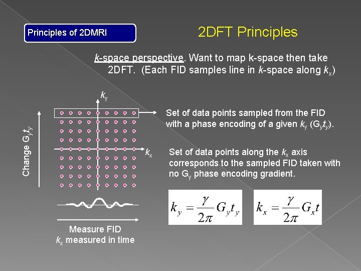
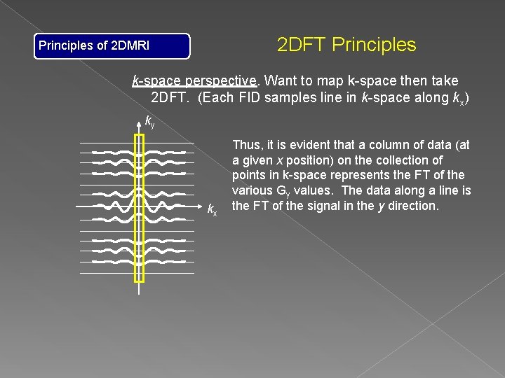
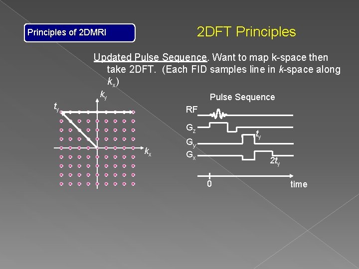
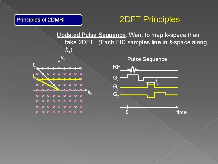
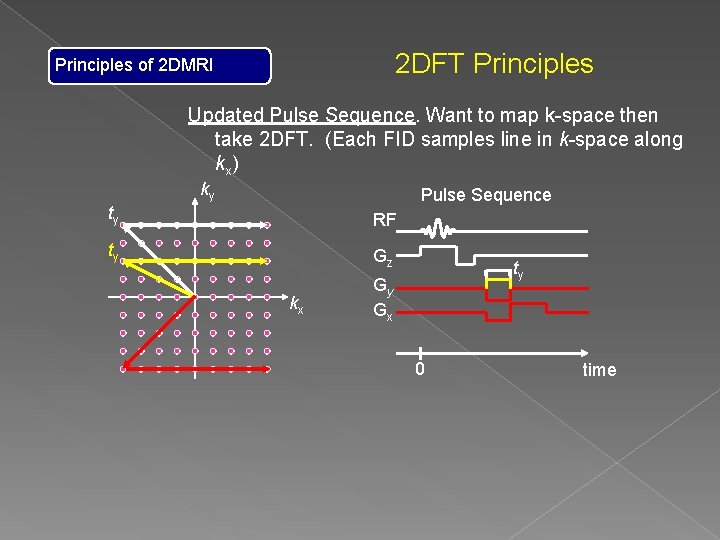
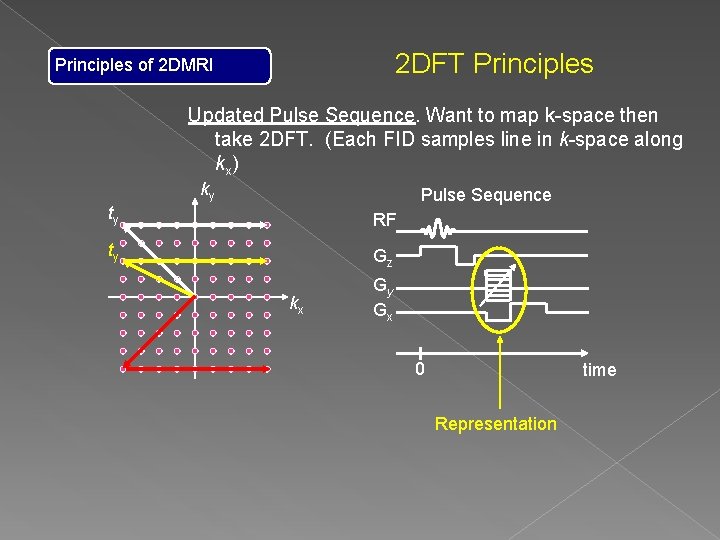
2 DFT Principles of 2 DMRI k-space perspective. Want to map k-space then take 2 DFT. (Each FID samples line in k-space along kx) ky Change Gyty Set of data points sampled from the FID with a phase encoding of a given ky (Gyty). kx Measure FID kx measured in time Set of data points along the kx axis corresponds to the sampled FID taken with no Gy phase encoding gradient.

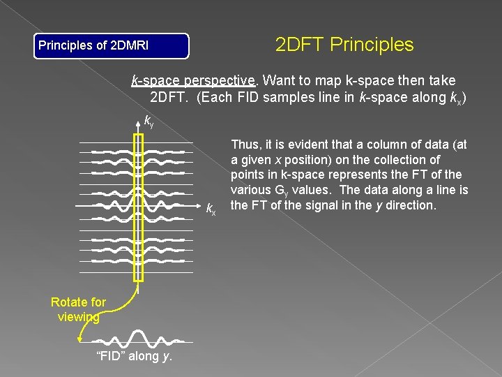
2 DFT Principles of 2 DMRI k-space perspective. Want to map k-space then take 2 DFT. (Each FID samples line in k-space along kx) ky kx Thus, it is evident that a column of data (at a given x position) on the collection of points in k-space represents the FT of the various Gy values. The data along a line is the FT of the signal in the y direction.

2 DFT Principles of 2 DMRI k-space perspective. Want to map k-space then take 2 DFT. (Each FID samples line in k-space along kx) ky kx Rotate for viewing “FID” along y. Thus, it is evident that a column of data (at a given x position) on the collection of points in k-space represents the FT of the various Gy values. The data along a line is the FT of the signal in the y direction.

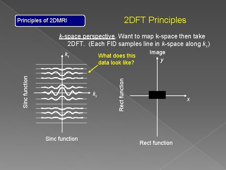
2 DFT Principles of 2 DMRI k-space perspective. Want to map k-space then take 2 DFT. (Each FID samples line in k-space along kx) What does this data look like? kx Sinc function Image y Rect function Sinc function ky x Rect function

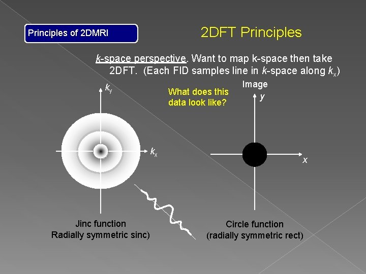
2 DFT Principles of 2 DMRI k-space perspective. Want to map k-space then take 2 DFT. (Each FID samples line in k-space along kx) ky What does this data look like? kx Jinc function Radially symmetric sinc) Image y x Circle function (radially symmetric rect)

2 DFT Principles of 2 DMRI Updated Pulse Sequence. Want to map k-space then take 2 DFT. (Each FID samples line in k-space along kx) ky Pulse Sequence ty RF Gz kx ty Gy Gx 2 ty 0 time

2 DFT Principles of 2 DMRI Updated Pulse Sequence. Want to map k-space then take 2 DFT. (Each FID samples line in k-space along kx) ky Pulse Sequence ty RF ty Gz kx ty Gy Gx 0 time

2 DFT Principles of 2 DMRI Updated Pulse Sequence. Want to map k-space then take 2 DFT. (Each FID samples line in k-space along kx) ky Pulse Sequence ty RF ty Gz kx ty Gy Gx 0 time

2 DFT Principles of 2 DMRI Updated Pulse Sequence. Want to map k-space then take 2 DFT. (Each FID samples line in k-space along kx) ky Pulse Sequence ty RF ty Gz kx Gy Gx 0 time Representation

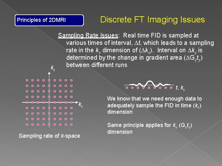
Discrete FT Imaging Issues Principles of 2 DMRI Sampling Rate Issues: Real time FID is sampled at various times of interval, Dt, which leads to a sampling rate in the kx dimension of (Dkx). Interval on Dky is determined by the change in gradient area (DGyty) between different runs ky t, kx kx Sampling rate of k-space We know that we need enough data to adequately sample the FID in time (kx) dimension Same principle applies for ky (Gyty) dimension

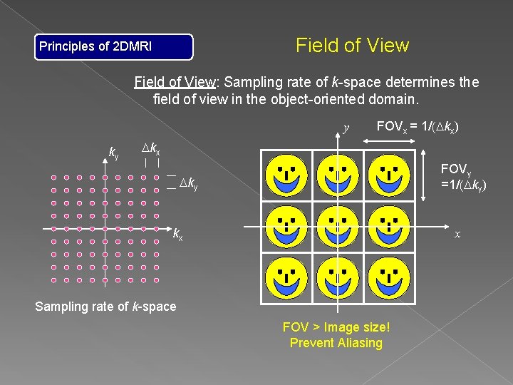
Field of View Principles of 2 DMRI Field of View: Sampling rate of k-space determines the field of view in the object-oriented domain. y ky FOVx = 1/(Dkx) Dkx FOVy =1/(Dky) Dky kx x Sampling rate of k-space FOV > Image size! Prevent Aliasing

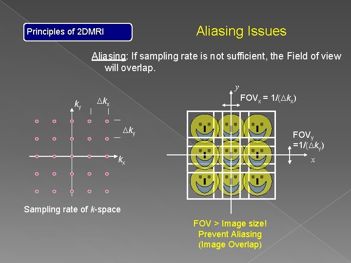
Aliasing Issues Principles of 2 DMRI Aliasing: If sampling rate is not sufficient, the Field of view will overlap. y ky FOVx = 1/(Dkx) Dkx Dky FOVy =1/(Dky) kx x Sampling rate of k-space FOV > Image size! Prevent Aliasing (Image Overlap)

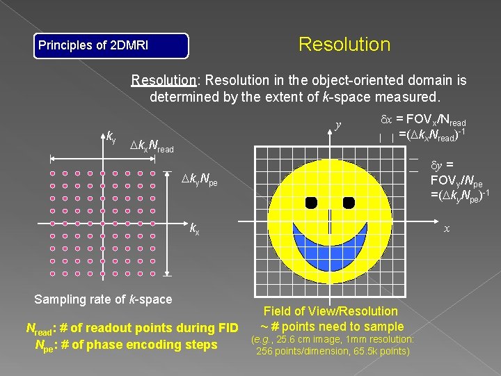
Resolution Principles of 2 DMRI Resolution: Resolution in the object-oriented domain is determined by the extent of k-space measured. ky y Dkx. Nread dx = FOVx/Nread =(Dkx. Nread)-1 dy = FOVy/Npe =(Dky. Npe)-1 Dky. Npe kx Sampling rate of k-space Nread: # of readout points during FID Npe: # of phase encoding steps x Field of View/Resolution ~ # points need to sample (e. g. , 25. 6 cm image, 1 mm resolution: 256 points/dimension, 65. 5 k points)

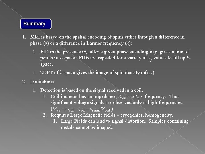
Summary 1. MRI is based on the spatial encoding of spins either through a difference in phase (y) or a difference in Larmor frequency (x): 1. FID in the presence Gx, after a given phase encoding in y, gives a line of points in k-space. FIDs are repeated for a variety of ky values to fill up kspace. 1. 2 DFT of k-space gives the image of spin density m(x, y) 2. Limitations. 1. Detection is based on the signal received in a coil. 1. Coil inductor has an impedance, Zcoil= iw. L, ~ frequency. Thus significant voltage signals are observed only at high frequencies. (Mxy → icoil = vsignal/Zcoil. ) 2. Requires Large Magnetic fields – cryogenics, homogeneity. 1. Large Fields can lead to signal distortion. Samples containing metals cannot be imaged.

Acknowledgements David Michalak Pines Group Budker Group Alex Pines Chip Crawford Hattie Ziegler Marcus Donaldson Thomas Theis All current ‘nuts Dmitry Budker Micah Ledbetter Good Books: 1) Principles of Magnetic Resonance Imaging, Dwight G. Nishimura, Stanford University 2) Magnetic Resonance Imaging: Physical Principles and Sequence Design, Haacke E. M. et al. , Wiley: New York, 1999.