PRINCIPLES OF EPIDEMIOLOGY DAVID R WOODARD MSC CIC

PRINCIPLES OF EPIDEMIOLOGY DAVID R. WOODARD, MSC, CIC, FSHEA

OBJECTIVES Define the term epidemiology Explain the elements involved in the transmission of infection Describe basic epidemiologic methods and study design Compute basic descriptive statistics and explore data analytic methods and displays

EPIDEMIOLOGY • The study of the distribution and determinants of disease and other conditions in specified populations in terms of: • Person • Place • Time • Natural history • Both a body of knowledge and a method of study

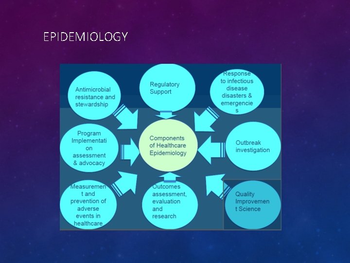
EPIDEMIOLOGY

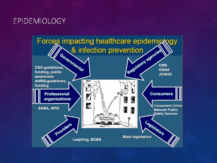
EPIDEMIOLOGY

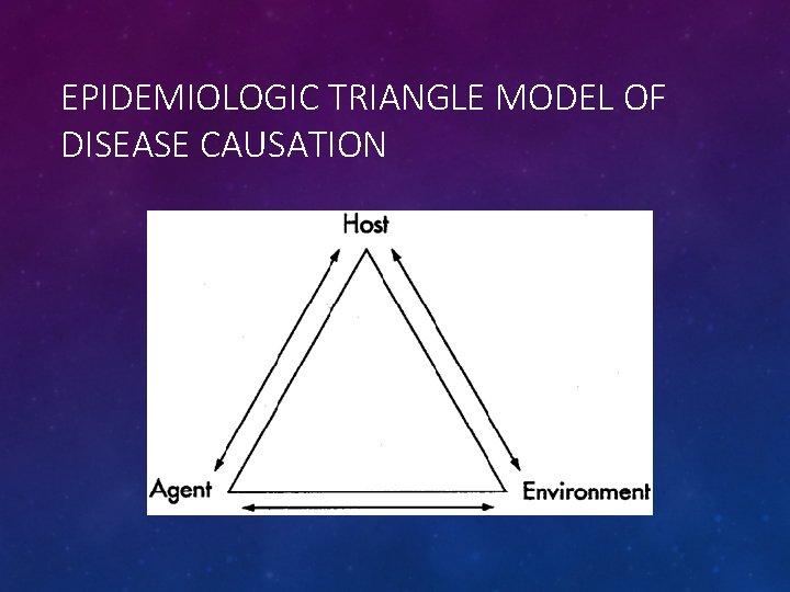
EPIDEMIOLOGIC TRIANGLE MODEL OF DISEASE CAUSATION

ASSOCIATION AND CAUSATION • Association – as one variable changes, there is a concomitant or resultant change in the quantity or quality of the other variable • Causation – one factor is clearly shown to increase the probability of occurrence of a disease • Statistics -- do not PROVE causality; they can merely suggest that an association exists

DEFINITIONS • Incidence - # of new cases of disease in a given time period • Prevalence - # of existing cases, events or conditions occurring in a population • Endemic – usual presence of disease or condition in a specific population or geographic area • Epidemic – occurrence of more cases of a disease than expected in a given area or among a specific group of people during a specific time period • Synonymous with “outbreak”

DEFINITIONS • Pandemic – epidemic spread over a wide geographic area, across countries or continents • Reservoir – place where an infectious agent can survive, but may not multiply • Fomite – inanimate object on which organisms may exist for some period of time

DEFINITIONS • Herd immunity – resistance of a group to invasion and spread of an infection • Based on the immunity of a high proportion of members of the group • Risk – probability or likelihood of an event occurring • Risk factor – characteristic, behavior or experience that increases the likelihood of a negative health status

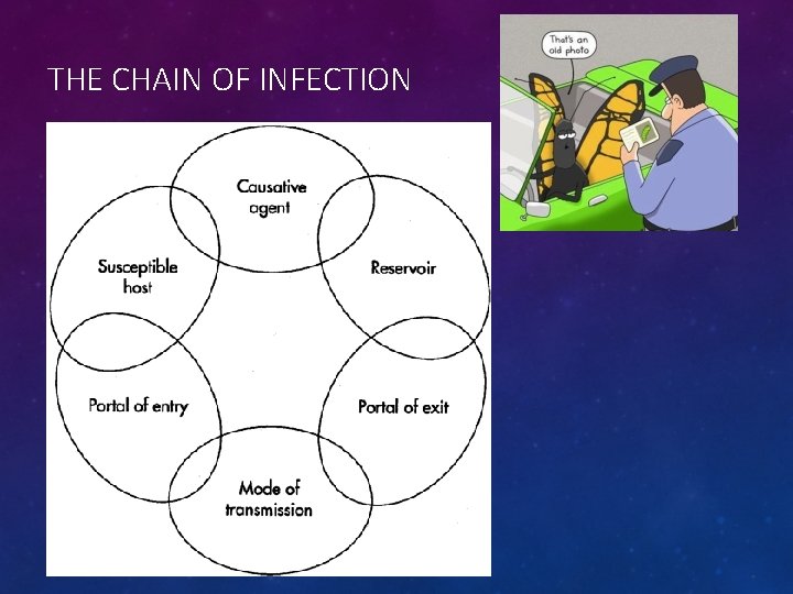
THE CHAIN OF INFECTION

BREAKING THE CHAIN – EPIDEMIOLOGIC STUDY DESIGNS • Observational – investigator does not intervene or control exposures or risk factors for study subjects • Descriptive • Person, place and time (e. g. , describe series of patients with a disorder including characteristics and outcomes) • Case studies, case reports • Analytic • Cohort • Case-control • Cross-sectional

ANALYTIC STUDIES • Cohort • Prospective or longitudinal • Population is free of the disease under study and is followed for exposure to risk factors and appearance of disease • Subjects form a “cohort” going through time together • Stronger evidence of causal association but more difficult, time consuming and expensive

ANALYTIC STUDIES • Case-control • Retrospective (Trohoc) • Start with a number of identified cases of the disease and compare them in terms of past exposures with a group of control subjects without the disease • Data already available, e. g. , charts, labs, etc. • Quicker, less expensive and easier

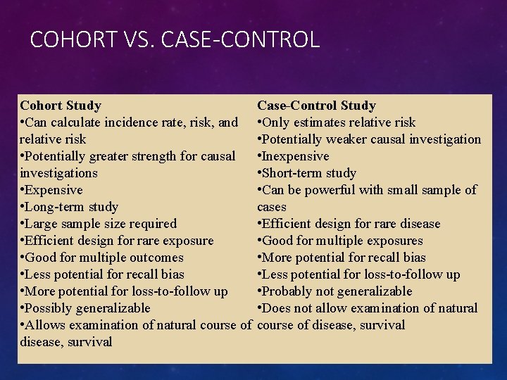
COHORT VS. CASE-CONTROL Cohort Study • Can calculate incidence rate, risk, and relative risk • Potentially greater strength for causal investigations • Expensive • Long-term study • Large sample size required • Efficient design for rare exposure • Good for multiple outcomes • Less potential for recall bias • More potential for loss-to-follow up • Possibly generalizable • Allows examination of natural course of disease, survival Case-Control Study • Only estimates relative risk • Potentially weaker causal investigation • Inexpensive • Short-term study • Can be powerful with small sample of cases • Efficient design for rare disease • Good for multiple exposures • More potential for recall bias • Less potential for loss-to-follow up • Probably not generalizable • Does not allow examination of natural course of disease, survival

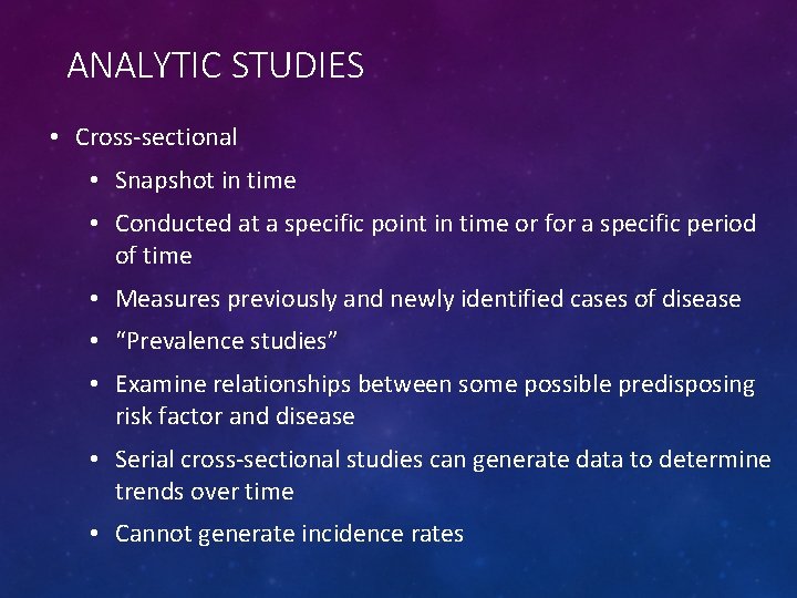
ANALYTIC STUDIES • Cross-sectional • Snapshot in time • Conducted at a specific point in time or for a specific period of time • Measures previously and newly identified cases of disease • “Prevalence studies” • Examine relationships between some possible predisposing risk factor and disease • Serial cross-sectional studies can generate data to determine trends over time • Cannot generate incidence rates

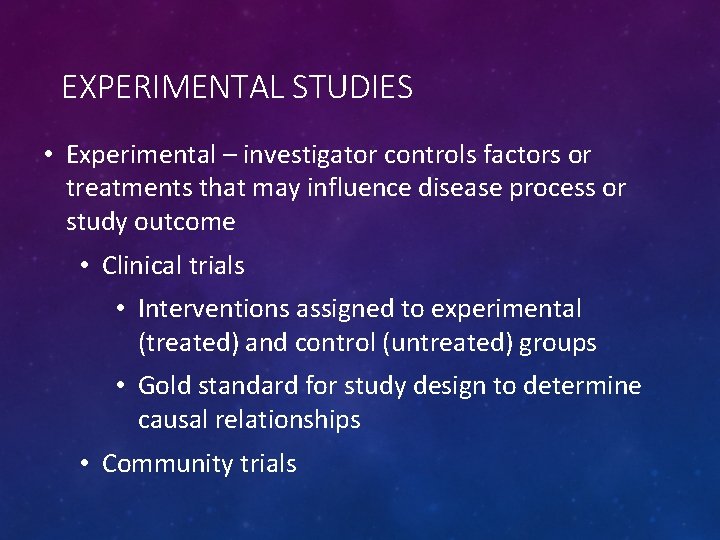
EXPERIMENTAL STUDIES • Experimental – investigator controls factors or treatments that may influence disease process or study outcome • Clinical trials • Interventions assigned to experimental (treated) and control (untreated) groups • Gold standard for study design to determine causal relationships • Community trials

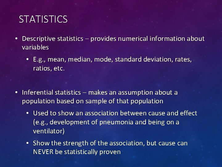
STATISTICS • Descriptive statistics – provides numerical information about variables • E. g. , mean, median, mode, standard deviation, rates, ratios, etc. • Inferential statistics – makes an assumption about a population based on sample of that population • Used to show an association between cause and effect (e. g. , development of pneumonia and being on a ventilator) • Show the strength of the association, but cause can NEVER be statistically proven

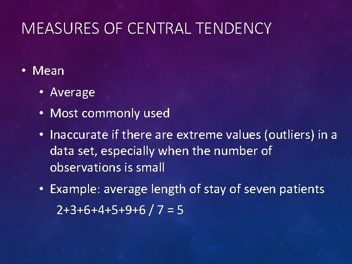
MEASURES OF CENTRAL TENDENCY • Mean • Average • Most commonly used • Inaccurate if there are extreme values (outliers) in a data set, especially when the number of observations is small • Example: average length of stay of seven patients 2+3+6+4+5+9+6 / 7 = 5

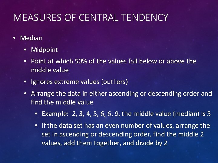
MEASURES OF CENTRAL TENDENCY • Median • Midpoint • Point at which 50% of the values fall below or above the middle value • Ignores extreme values (outliers) • Arrange the data in either ascending or descending order and find the middle value • Example: 2, 3, 4, 5, 6, 6, 9, the middle value (median) is 5 • If the data set has an even number of values, arrange the set in ascending or descending order, find the middle 2 values, add them together, and divide by 2

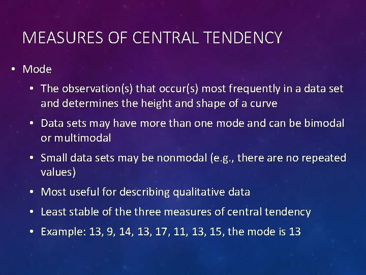
MEASURES OF CENTRAL TENDENCY • Mode • The observation(s) that occur(s) most frequently in a data set and determines the height and shape of a curve • Data sets may have more than one mode and can be bimodal or multimodal • Small data sets may be nonmodal (e. g. , there are no repeated values) • Most useful for describing qualitative data • Least stable of the three measures of central tendency • Example: 13, 9, 14, 13, 17, 11, 13, 15, the mode is 13

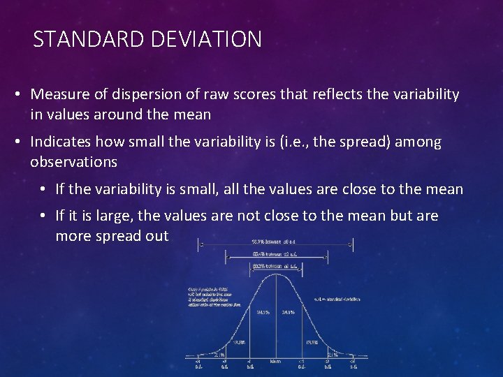
STANDARD DEVIATION • Measure of dispersion of raw scores that reflects the variability in values around the mean • Indicates how small the variability is (i. e. , the spread) among observations • If the variability is small, all the values are close to the mean • If it is large, the values are not close to the mean but are more spread out

RELIABILITY • Sensitivity • Probability of a positive test among patients with disease • A high sensitivity test is when a negative rules out disease • Specificity • Probability of a negative test among patients without disease • A high specificity test is when a positive rules in disease

RATES • Expression of frequency with which an event occurs in a defined population per unit of time • Rate = x/y × k • x = The numerator, which equals the number of times the event (e. g. , infections) has occurred during a specified time interval • y = The denominator, which equals a population (e. g. , number of patients at risk) from which those experiencing the event were derived during the same time interval

RATES • k = A constant used to transform the result of division into a uniform quantity so that it can be compared with other, similar quantities • Selection of k is usually made so that the smallest rate calculated has at least one digit to the left of the decimal point, or is determined by accepted practice • CLABSI rates: # infections/# line days x 1000 • CDI rate: # infections/# patient days x 10, 000

RATES • Rules for rates: • Persons in the denominator must reflect the same population from which the numerator was taken • Counts in the numerator and denominator should cover the same time period • At least in theory, the persons in the denominator should have been at risk of the event or occurrence

INCIDENCE RATES • # of new cases of a disease for a specified time period / population at risk for the same time period x a constant • x/y × k • x is the number of new cases or events in a population during a given time period • y is the number in the population at risk during that time period • k is used to transform the result into a number that has at least one digit to the left of the decimal point

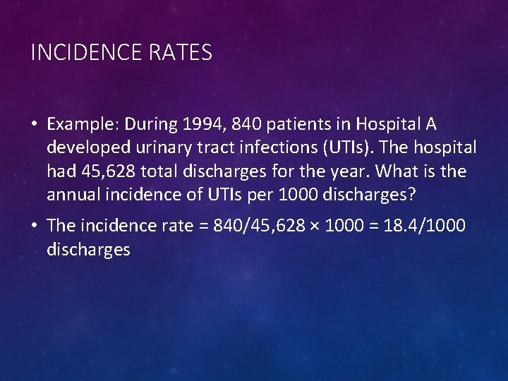
INCIDENCE RATES • Example: During 1994, 840 patients in Hospital A developed urinary tract infections (UTIs). The hospital had 45, 628 total discharges for the year. What is the annual incidence of UTIs per 1000 discharges? • The incidence rate = 840/45, 628 × 1000 = 18. 4/1000 discharges

PREVALENCE RATES • Proportion of persons in a population with an existing case of disease or attribute at a specific point in time (point prevalence) or over a specified time period (period prevalence) • # of existing cases of disease from a specified interval or point in time / population at risk for same time period x a constant • x/y × k

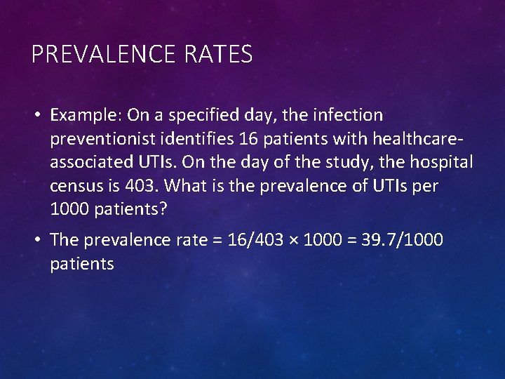
PREVALENCE RATES • Example: On a specified day, the infection preventionist identifies 16 patients with healthcareassociated UTIs. On the day of the study, the hospital census is 403. What is the prevalence of UTIs per 1000 patients? • The prevalence rate = 16/403 × 1000 = 39. 7/1000 patients

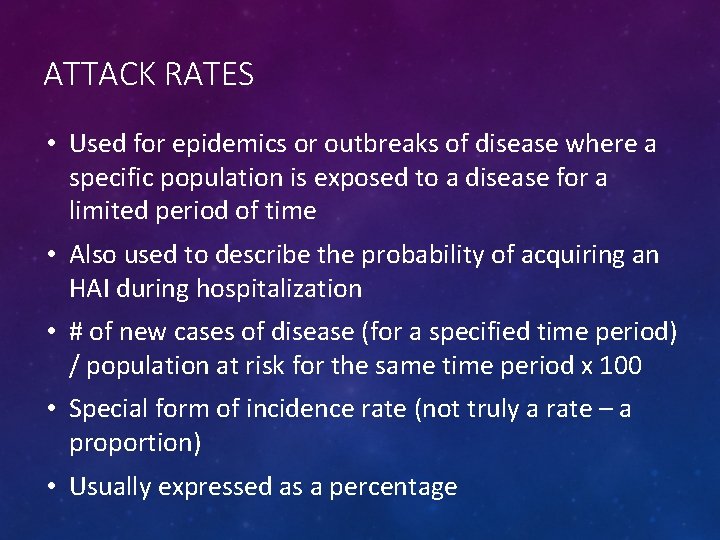
ATTACK RATES • Used for epidemics or outbreaks of disease where a specific population is exposed to a disease for a limited period of time • Also used to describe the probability of acquiring an HAI during hospitalization • # of new cases of disease (for a specified time period) / population at risk for the same time period x 100 • Special form of incidence rate (not truly a rate – a proportion) • Usually expressed as a percentage

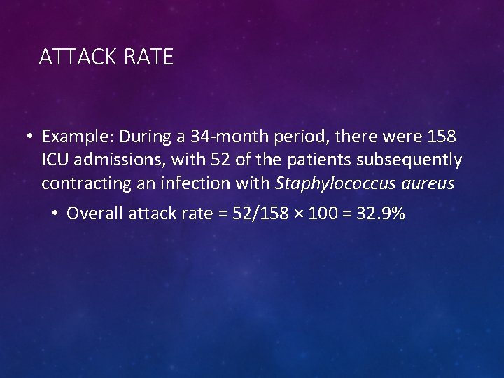
ATTACK RATE • Example: During a 34 -month period, there were 158 ICU admissions, with 52 of the patients subsequently contracting an infection with Staphylococcus aureus • Overall attack rate = 52/158 × 100 = 32. 9%

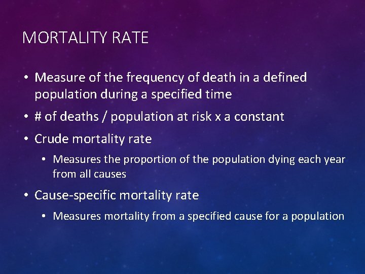
MORTALITY RATE • Measure of the frequency of death in a defined population during a specified time • # of deaths / population at risk x a constant • Crude mortality rate • Measures the proportion of the population dying each year from all causes • Cause-specific mortality rate • Measures mortality from a specified cause for a population

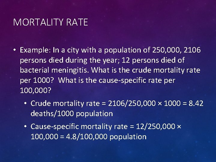
MORTALITY RATE • Example: In a city with a population of 250, 000, 2106 persons died during the year; 12 persons died of bacterial meningitis. What is the crude mortality rate per 1000? What is the cause-specific rate per 100, 000? • Crude mortality rate = 2106/250, 000 × 1000 = 8. 42 deaths/1000 population • Cause-specific mortality rate = 12/250, 000 × 100, 000 = 4. 8/100, 000 population

RISK RATIO (RR) • Probability of developing a disease if the risk factor is present / probability of developing disease if the risk factor is not present • Measure of the strength of association used in prospective (cohort) and experimental studies (based on incidence) • Asks the question: What is the risk of developing disease if exposed to the risk factor?

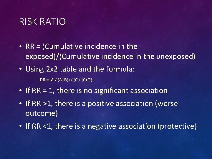
RISK RATIO • RR = (Cumulative incidence in the exposed)/(Cumulative incidence in the unexposed) • Using 2 x 2 table and the formula: RR = (A / (A+B)) / (C+D)) • If RR = 1, there is no significant association • If RR >1, there is a positive association (worse outcome) • If RR <1, there is a negative association (protective)

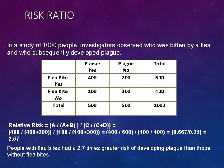
RISK RATIO In a study of 1000 people, investigators observed who was bitten by a flea and who subsequently developed plague. Flea Bite Yes Flea Bite No Total Plague Yes 400 Plague No 200 Total 100 300 400 500 1000 600 Relative Risk = (A / (A+B) ) / (C+D)) = (400 / (400+200)) / (100+300)) = (400 / 600) / (100 / 400) = (0. 667/0. 25) = 2. 67 People with flea bites had a 2. 7 times greater risk of developing plague than those without flea bites.

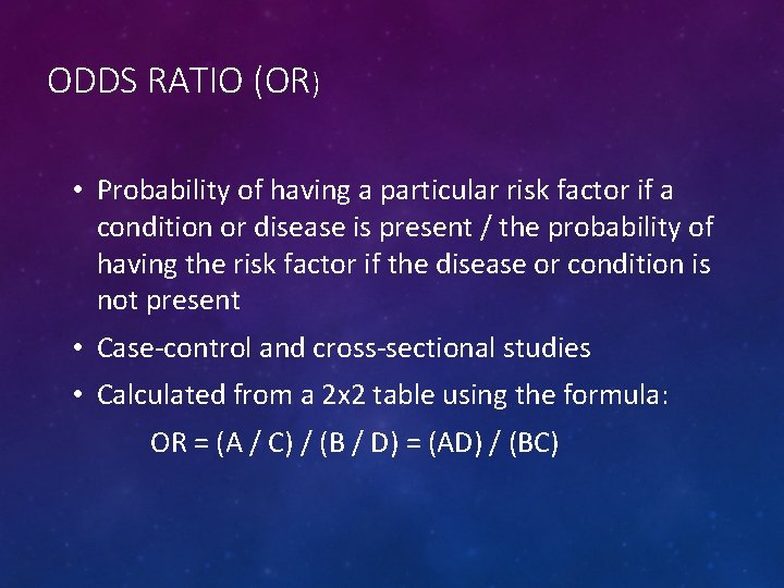
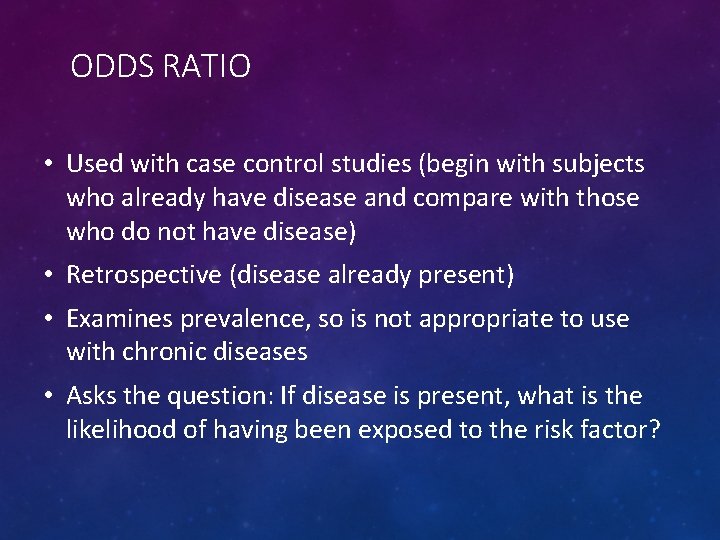
ODDS RATIO (OR) • Probability of having a particular risk factor if a condition or disease is present / the probability of having the risk factor if the disease or condition is not present • Case-control and cross-sectional studies • Calculated from a 2 x 2 table using the formula: OR = (A / C) / (B / D) = (AD) / (BC)

ODDS RATIO • Used with case control studies (begin with subjects who already have disease and compare with those who do not have disease) • Retrospective (disease already present) • Examines prevalence, so is not appropriate to use with chronic diseases • Asks the question: If disease is present, what is the likelihood of having been exposed to the risk factor?

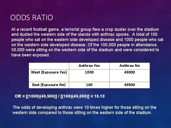
ODDS RATIO At a recent football game, a terrorist group flew a crop duster over the stadium and dusted the western side of the stands with anthrax spores. A total of 100 people who sat on the eastern side developed disease and 1000 people who sat on the western side developed disease. Of the 100, 000 people in attendance, 50, 000 were sitting on the western side of the stadium and were considered to have been exposed. Anthrax Yes Anthrax No West (Exposure Yes) 1000 49000 East (Exposure No) 100 49900 OR = [(1000)(49, 900)] / [(100)(49, 000)] = 10. 18 The odds of developing anthrax were 10 times higher for those sitting on the western side compared to those sitting on the eastern side of the stadium.

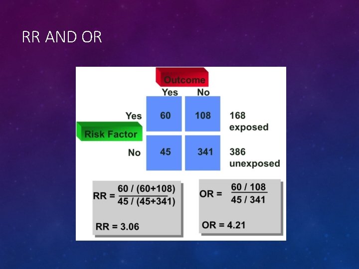
RR AND OR

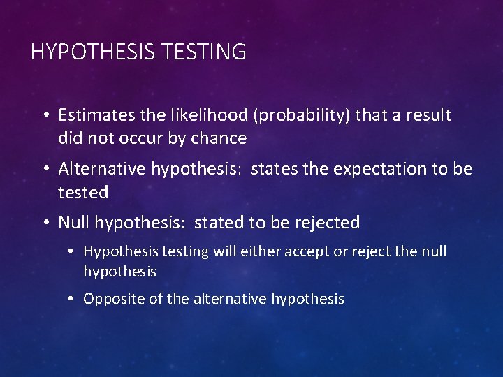
HYPOTHESIS TESTING • Estimates the likelihood (probability) that a result did not occur by chance • Alternative hypothesis: states the expectation to be tested • Null hypothesis: stated to be rejected • Hypothesis testing will either accept or reject the null hypothesis • Opposite of the alternative hypothesis

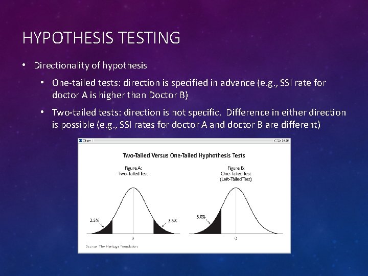
HYPOTHESIS TESTING • Directionality of hypothesis • One-tailed tests: direction is specified in advance (e. g. , SSI rate for doctor A is higher than Doctor B) • Two-tailed tests: direction is not specific. Difference in either direction is possible (e. g. , SSI rates for doctor A and doctor B are different)

HYPOTHESIS TESTING • Type I (α) error • Probability of rejecting a true null hypothesis and attributing significance when there is none • Indicates the significance level, or p value • Usually set to 0. 05 • Type II (β) error • Accepting the null hypothesis when it is false or not attributing significance when it exists • Heavily influenced by sample size

HYPOTHESIS TESTING • Control • Keeping α level very small (e. g. , 0. 05 or 0. 01) decreases the risk for committing a type I error • No control over type II error except sample size (e. g. , increase sample size to decrease error) • Type I and II errors are inversely related • Once the sample size is fixed, decreasing the risk for committing a type I error increases the risk of committing a type II error • Impossible to control both simultaneously

PARAMETRIC TESTS • Z test • Most appropriate to test that the means of two samples are not different (two-tailed hypothesis) • Requires a normal distribution and a sample size of 30 or more • Example: compare the mean of infection rates against the NHSN mean or another benchmark mean

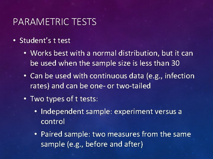
PARAMETRIC TESTS • Student’s t test • Works best with a normal distribution, but it can be used when the sample size is less than 30 • Can be used with continuous data (e. g. , infection rates) and can be one- or two-tailed • Two types of t tests: • Independent sample: experiment versus a control • Paired sample: two measures from the sample (e. g. , before and after)

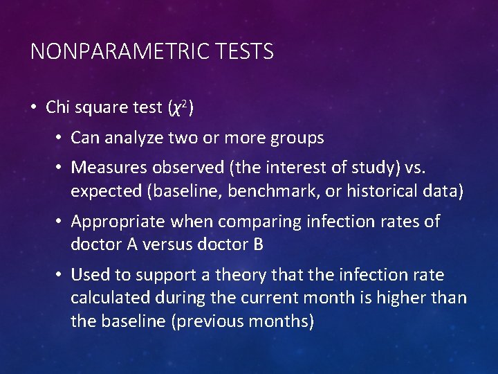
NONPARAMETRIC TESTS • Chi square test (χ2) • Can analyze two or more groups • Measures observed (the interest of study) vs. expected (baseline, benchmark, or historical data) • Appropriate when comparing infection rates of doctor A versus doctor B • Used to support a theory that the infection rate calculated during the current month is higher than the baseline (previous months)

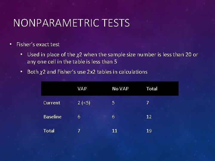
NONPARAMETRIC TESTS • Fisher’s exact test • Used in place of the χ2 when the sample size number is less than 20 or any one cell in the table is less than 5 • Both χ2 and Fisher’s use 2 x 2 tables in calculations VAP No VAP Total Current 2 (<5) 5 7 Baseline 6 6 12 Total 7 11 19

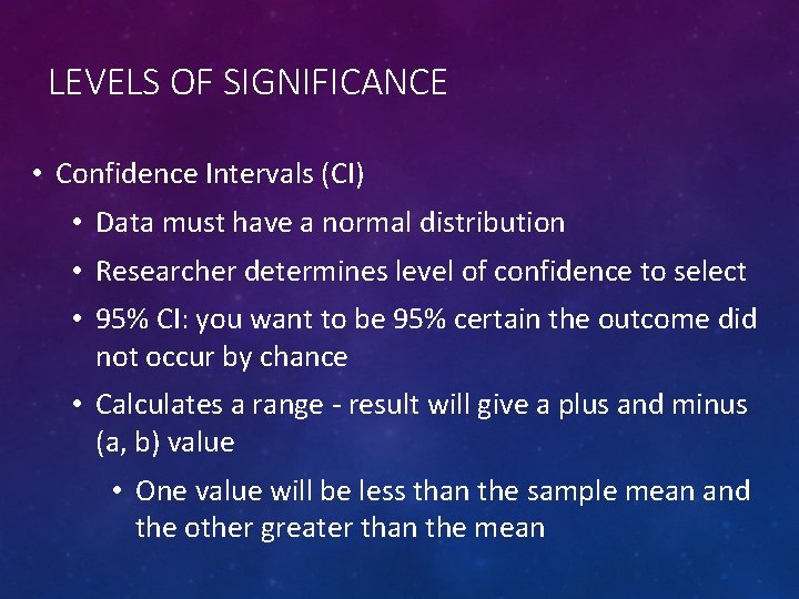
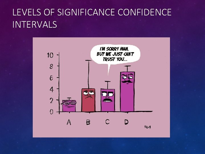
LEVELS OF SIGNIFICANCE • Confidence Intervals (CI) • Data must have a normal distribution • Researcher determines level of confidence to select • 95% CI: you want to be 95% certain the outcome did not occur by chance • Calculates a range - result will give a plus and minus (a, b) value • One value will be less than the sample mean and the other greater than the mean

LEVELS OF SIGNIFICANCE CONFIDENCE INTERVALS

LEVELS OF SIGNIFICANCE • p Value • Probability of an event occurring due to chance alone • The higher the p-value, the higher the probability that the event you are observing can be explained by chance • p-values of either 0. 05 or 0. 01 are usually used as a cutoff value, although this value is arbitrary • Results larger than the cutoff are considered likely to attribute the event to chance, while results smaller than the cutoff value are likely to have occurred because of a real explanation • Type 1 (α) errors

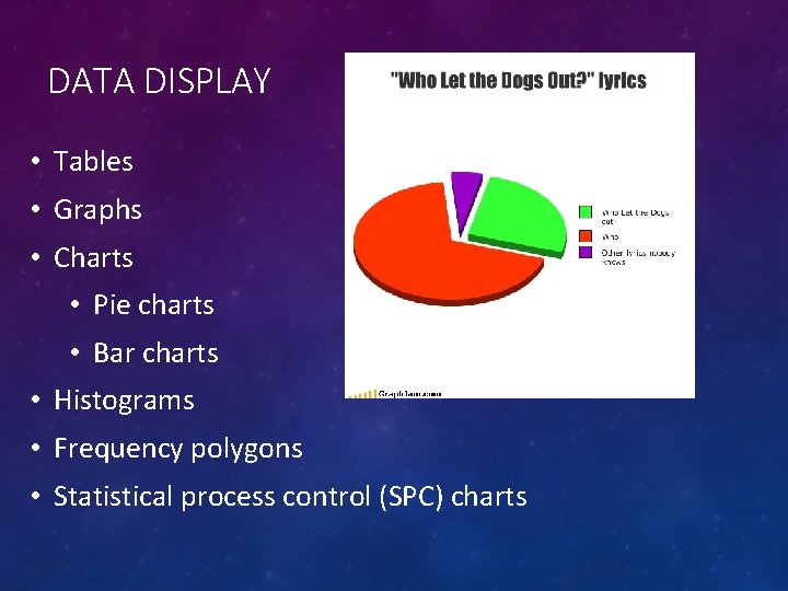
DATA DISPLAY • Tables • Graphs • Charts • Pie charts • Bar charts • Histograms • Frequency polygons • Statistical process control (SPC) charts

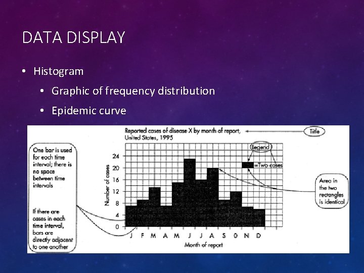
DATA DISPLAY • Histogram • Graphic of frequency distribution • Epidemic curve

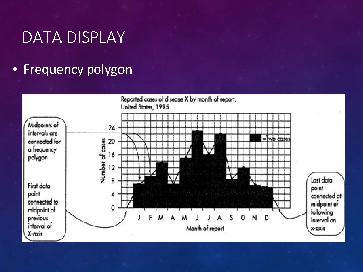
DATA DISPLAY • Frequency polygon • Similar to a line graph, but each coordinate point is represented by a point displayed on the graph with straight lines connecting them • Provides the same data information as a histogram • Can use line and points instead of bars • Can show two sets of data on one graph

DATA DISPLAY • Frequency polygon

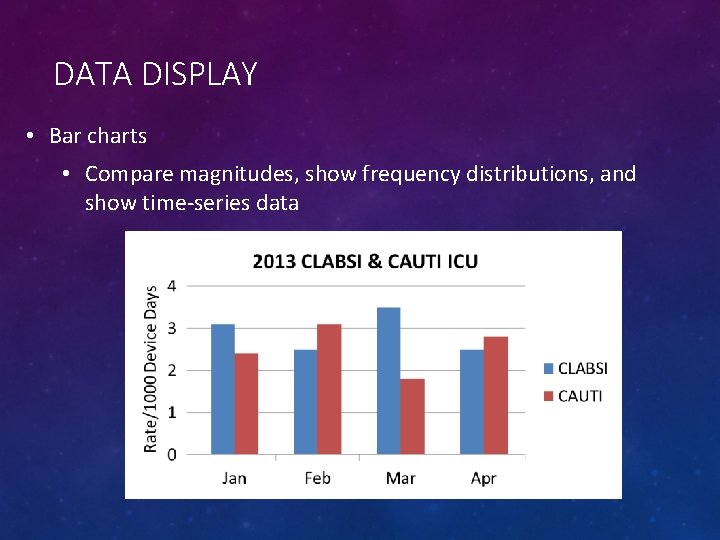
DATA DISPLAY • Bar charts • Compare magnitudes, show frequency distributions, and show time-series data

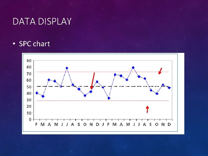
DATA DISPLAY • Statistical Process Control (SPC) charts • Range of expected variation about a mean (centerline) • Upper control limit (UCL) and lower control limit (LCL) beyond which the process is considered out of control • Control limits - three standard deviations above and below the mean • Changes in rates over time and identifying points in time when infection rates or other processes are outside the expected range • Processes that are out of control (i. e. , increasing infection rate) can be identified, and prevention efforts put in place to regain control

DATA DISPLAY • SPC chart UCL Mean LCL

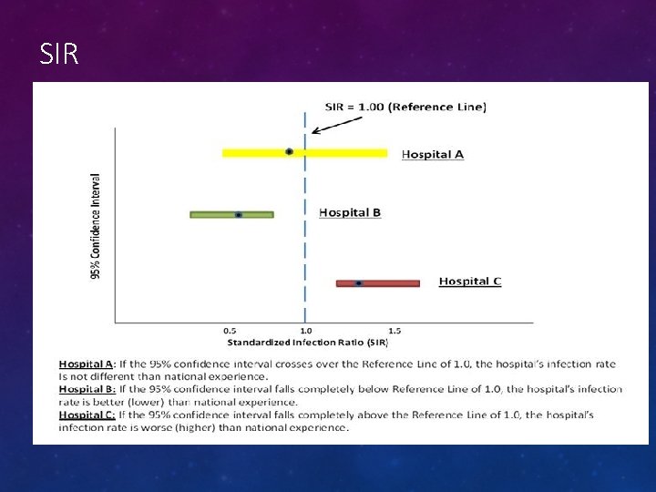
STANDARDIZED INFECTION RATIO (SIR) • Alternative to calculating rates • Same data, different method • Compare actual numbers of infections with corresponding standardized, risk adjusted predicted number of infections • Observed vs. Predicted numbers of infections • Expressed as a ratio • Standardized Infection Ratio, or SIR

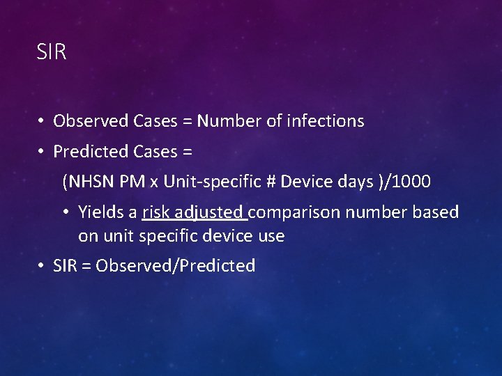
SIR • Observed Cases = Number of infections • Predicted Cases = (NHSN PM x Unit-specific # Device days )/1000 • Yields a risk adjusted comparison number based on unit specific device use • SIR = Observed/Predicted

SIR • The SIR value will be from ZERO to 1 and above • A value LESS than 1 indicates that observed cases were LOWER than expected (Desirable) • SIR = 0. 75 = Performing at 25% lower than comparable groups • A value of 1 indicates that observed cases were EQUAL to expected

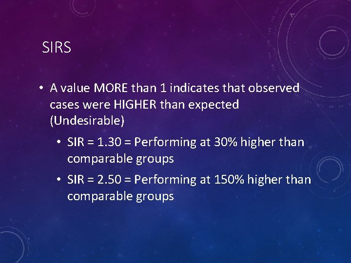
SIRS • A value MORE than 1 indicates that observed cases were HIGHER than expected (Undesirable) • SIR = 1. 30 = Performing at 30% higher than comparable groups • SIR = 2. 50 = Performing at 150% higher than comparable groups

SIRS – AS AN OUTCOME • Goal/Objective • “I want my SIR to be 0. 5” • What that means – ”I’m perfectly happy being an “average” hospital”

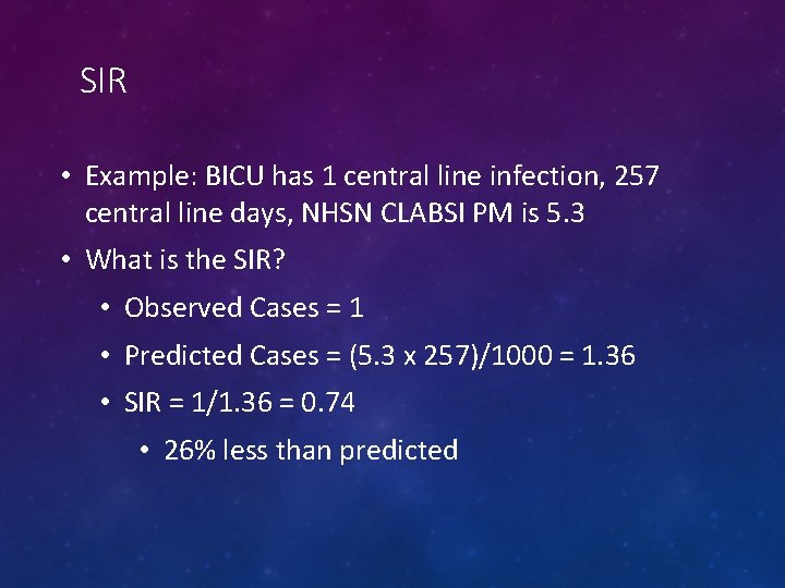
SIR • Example: BICU has 1 central line infection, 257 central line days, NHSN CLABSI PM is 5. 3 • What is the SIR? • Observed Cases = 1 • Predicted Cases = (5. 3 x 257)/1000 = 1. 36 • SIR = 1/1. 36 = 0. 74 • 26% less than predicted

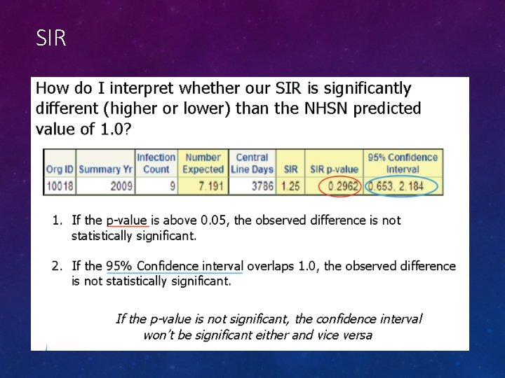
SIR

SIR

SIR

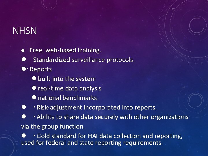
NHSN Free, web-based training. Standardized surveillance protocols. Reports built into the system real-time data analysis national benchmarks. Risk-adjustment incorporated into reports. Ability to share data securely with other organizations via the group function. Gold standard for HAI data collection and reporting, used for federal and state reporting requirements.

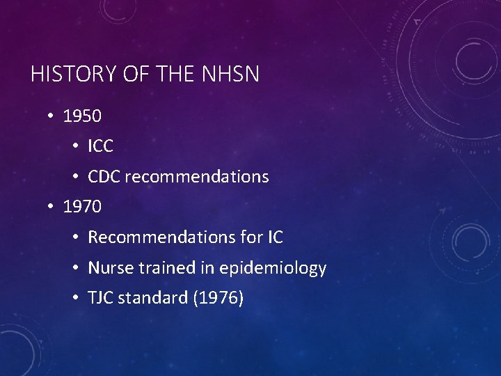
HISTORY OF THE NHSN • 1950 • ICC • CDC recommendations • 1970 • Recommendations for IC • Nurse trained in epidemiology • TJC standard (1976)

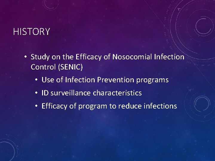
HISTORY • Study on the Efficacy of Nosocomial Infection Control (SENIC) • Use of Infection Prevention programs • ID surveillance characteristics • Efficacy of program to reduce infections

HISTORY • National Nosocomial Infections Surveillance • 1970 -2004 • 62 hospitals > 320 • Critical Care foundation • Trained ICP • Large and academic facilities

NNIS • Descriptive information (why we exist) • Developed sound model for surveillance • Established rates for comparative data • Standardized definitions and protocols • Electronic data submission • Aggregated data

NSHN • 2004 • Minimize data collection and manual data entry! • Data sharing • No FTE requirements

NHSN § Ability to share data securely with other organizations via the group function § Gold standard for HAI data collection and reporting, used for federal and state reporting requirements. § Standardized case definitions

DATA VALIDATION • Third party duties • CLABSI • SSI • CAUTI • Tri-annual • ? Internal validation

QUESTIONS? Resources: • APIC Online Text: • http: //text. apic. org/item-3/chapter-2 -general-principlesepidemiology/all • http: //text. apic. org/item-6/chapter-5 -use-of-statistics/all • http: //text. apic. org/item-7/chapter-6 -statistical-process-control • CDC • http: //www. cdc. gov/learning/resources/epidemiology. html • Thanks to JC – friend, colleague, professional

THE END