PRINCIPLES OF ECONOMICS Third Edition Oxford Fajar Sdn

PRINCIPLES OF ECONOMICS Third Edition © Oxford Fajar Sdn. Bhd. (008974 -T), 2013 All Rights Reserved 4– 1

CHAPTER 4 THEORY OF CONSUMER BEHAVIOUR PRINCIPLES OF ECONOMICS Third Edition © Oxford Fajar Sdn. Bhd. (008974 -T), 2013 All Rights Reserved 4– 2

DEFINITION OF CONSUMER BEHAVIOUR Consumer behaviour refers to the study of consumer while engaged in the process of consumption. PRINCIPLES OF ECONOMICS Third Edition © Oxford Fajar Sdn. Bhd. (008974 -T), 2013 All Rights Reserved 4– 3

UTILITY APPROACH q q Definition – ‘Utility’ means the satisfaction obtained from consuming a commodity. Two Types of Approach – Cardinal Approach • The cardinal utility theory says that utility is measurable and by placing a number of alternatives so that the utility can be added. • The index used to measure utility is called utils. – Ordinal Approach • The ordinal utility theory says that utility is not measurable but it can be compared. • Ordinal approach uses the ranking of alternatives as first, second, third and so on. PRINCIPLES OF ECONOMICS Third Edition © Oxford Fajar Sdn. Bhd. (008974 -T), 2013 All Rights Reserved 4– 4

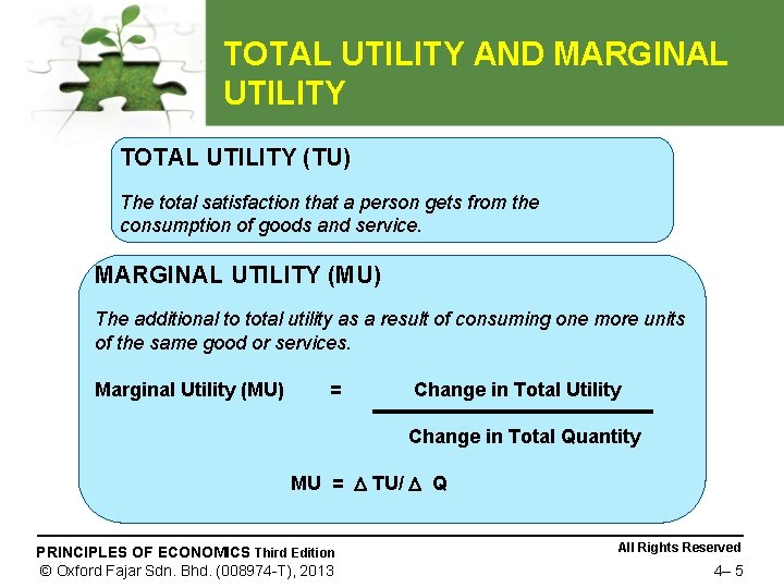
TOTAL UTILITY AND MARGINAL UTILITY TOTAL UTILITY (TU) The total satisfaction that a person gets from the consumption of goods and service. MARGINAL UTILITY (MU) The additional to total utility as a result of consuming one more units of the same good or services. Marginal Utility (MU) = Change in Total Utility Change in Total Quantity MU = TU/ Q PRINCIPLES OF ECONOMICS Third Edition © Oxford Fajar Sdn. Bhd. (008974 -T), 2013 All Rights Reserved 4– 5

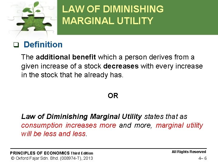
LAW OF DIMINISHING MARGINAL UTILITY q Definition The additional benefit which a person derives from a given increase of a stock decreases with every increase in the stock that he already has. OR Law of Diminishing Marginal Utility states that as consumption increases more and more, marginal utility will be less and less. PRINCIPLES OF ECONOMICS Third Edition © Oxford Fajar Sdn. Bhd. (008974 -T), 2013 All Rights Reserved 4– 6

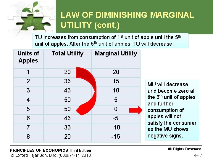
LAW OF DIMINISHING MARGINAL UTILITY (cont. ) TU increases from consumption of 1 st unit of apple until the 5 th unit of apples. After the 5 th unit of apples, TU will decrease. Units of Apples Total Utility Marginal Utility 1 20 20 2 35 15 3 45 10 4 50 5 5 50 0 6 45 -5 7 35 -10 8 20 -15 PRINCIPLES OF ECONOMICS Third Edition © Oxford Fajar Sdn. Bhd. (008974 -T), 2013 MU will decrease and become zero at the 5 th unit of apples and further consumption of apples will not satisfy the consumer as the MU shows negative signs. All Rights Reserved 4– 7

LAW OF DIMINISHING MARGINAL UTILITY (cont. ) When TU is increasing, MU will be positive. When TU is at its maximum, MU will be zero. When TU is decreasing, MU will be negative. PRINCIPLES OF ECONOMICS Third Edition © Oxford Fajar Sdn. Bhd. (008974 -T), 2013 All Rights Reserved 4– 8

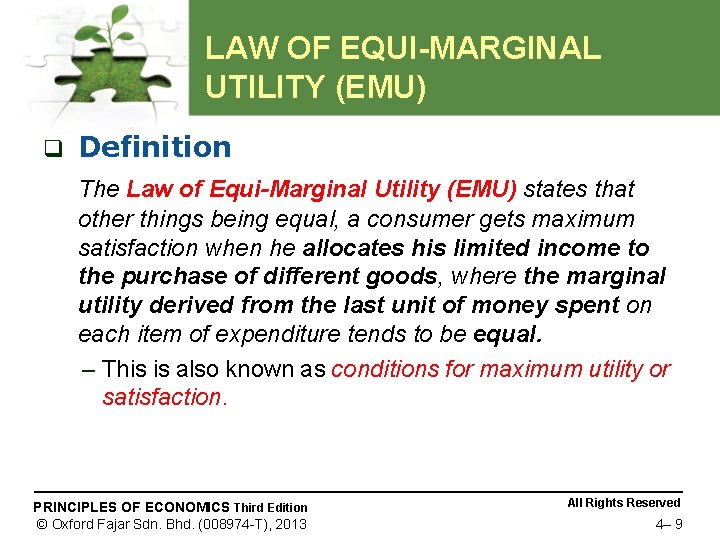
LAW OF EQUI-MARGINAL UTILITY (EMU) q Definition The Law of Equi-Marginal Utility (EMU) states that other things being equal, a consumer gets maximum satisfaction when he allocates his limited income to the purchase of different goods, where the marginal utility derived from the last unit of money spent on each item of expenditure tends to be equal. – This is also known as conditions for maximum utility or satisfaction. PRINCIPLES OF ECONOMICS Third Edition © Oxford Fajar Sdn. Bhd. (008974 -T), 2013 All Rights Reserved 4– 9

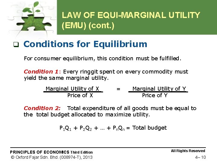
LAW OF EQUI-MARGINAL UTILITY (EMU) (cont. ) q Conditions for Equilibrium For consumer equilibrium, this condition must be fulfilled. Condition 1: Every ringgit spent on every commodity must yield the same marginal utility. Marginal Utility of X Price of X = Marginal Utility of Y Price of Y Condition 2: Total expenditure of all goods must be equal to the total budget allocated to maximize utility. P 1 Q 1 + P 2 Q 2 + … + Pn. Qn = Total budget PRINCIPLES OF ECONOMICS Third Edition © Oxford Fajar Sdn. Bhd. (008974 -T), 2013 All Rights Reserved 4– 10

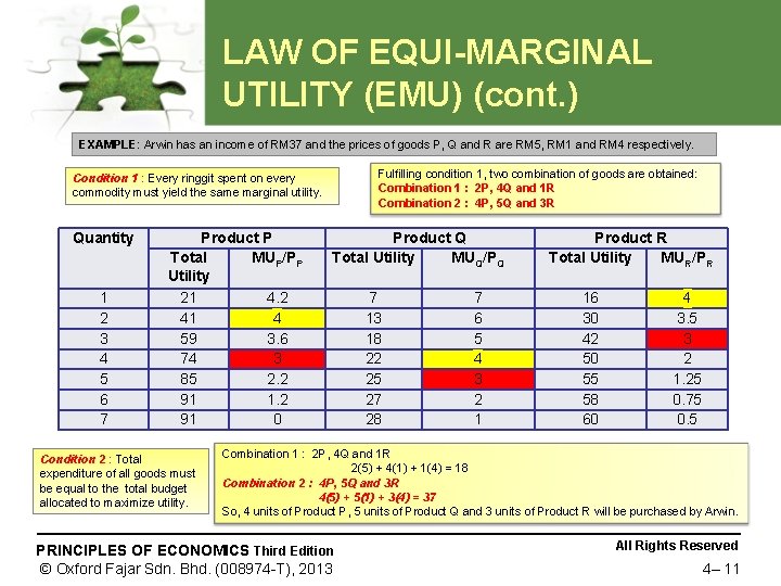
LAW OF EQUI-MARGINAL UTILITY (EMU) (cont. ) EXAMPLE: Arwin has an income of RM 37 and the prices of goods P, Q and R are RM 5, RM 1 and RM 4 respectively. Fulfilling condition 1, two combination of goods are obtained: Combination 1 : 2 P, 4 Q and 1 R Combination 2 : 4 P, 5 Q and 3 R Condition 1 : Every ringgit spent on every commodity must yield the same marginal utility. Quantity 1 2 3 4 5 6 7 Product P Total MUP/PP Utility 21 4. 2 41 4 59 3. 6 74 3 85 2. 2 91 1. 2 91 0 Condition 2 : Total expenditure of all goods must be equal to the total budget allocated to maximize utility. Product Q Total Utility MUQ/PQ 7 13 18 22 25 27 28 7 6 5 4 3 2 1 Product R Total Utility MUR/PR 16 30 42 50 55 58 60 4 3. 5 3 2 1. 25 0. 75 0. 5 Combination 1 : 2 P, 4 Q and 1 R 2(5) + 4(1) + 1(4) = 18 Combination 2 : 4 P, 5 Q and 3 R 4(5) + 5(1) + 3(4) = 37 So, 4 units of Product P, 5 units of Product Q and 3 units of Product R will be purchased by Arwin. PRINCIPLES OF ECONOMICS Third Edition © Oxford Fajar Sdn. Bhd. (008974 -T), 2013 All Rights Reserved 4– 11

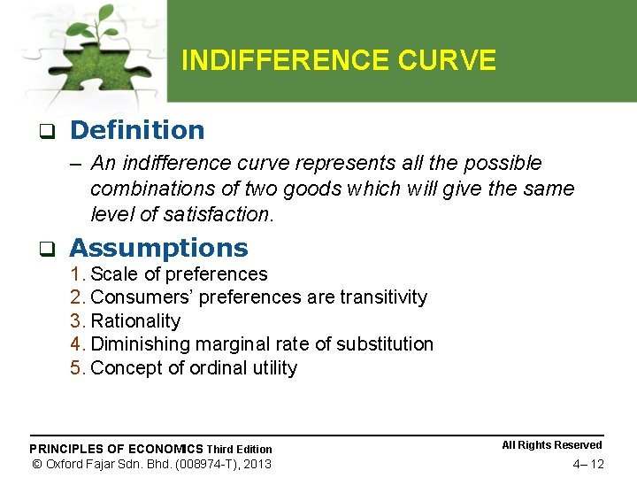
INDIFFERENCE CURVE q Definition – An indifference curve represents all the possible combinations of two goods which will give the same level of satisfaction. q Assumptions 1. Scale of preferences 2. Consumers’ preferences are transitivity 3. Rationality 4. Diminishing marginal rate of substitution 5. Concept of ordinal utility PRINCIPLES OF ECONOMICS Third Edition © Oxford Fajar Sdn. Bhd. (008974 -T), 2013 All Rights Reserved 4– 12

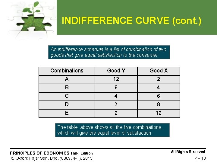
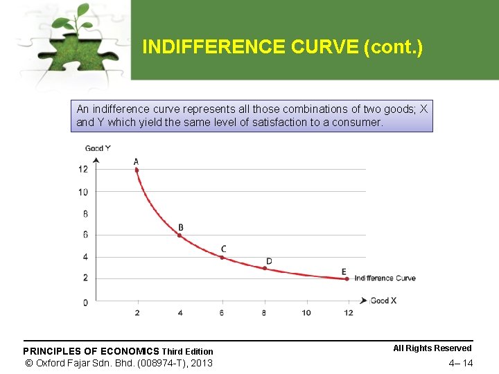
INDIFFERENCE CURVE (cont. ) An indifference schedule is a list of combination of two goods that give equal satisfaction to the consumer. Combinations Good Y Good X A 12 2 B 6 4 C 4 6 D 3 8 E 2 12 The table above shows all the five combinations, which will give the equal level of satisfaction. PRINCIPLES OF ECONOMICS Third Edition © Oxford Fajar Sdn. Bhd. (008974 -T), 2013 All Rights Reserved 4– 13

INDIFFERENCE CURVE (cont. ) An indifference curve represents all those combinations of two goods; X and Y which yield the same level of satisfaction to a consumer. PRINCIPLES OF ECONOMICS Third Edition © Oxford Fajar Sdn. Bhd. (008974 -T), 2013 All Rights Reserved 4– 14

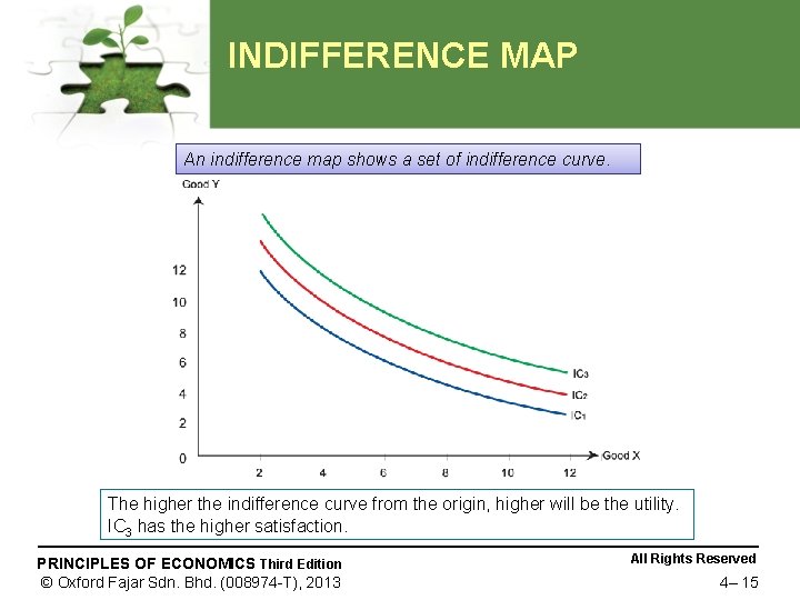
INDIFFERENCE MAP An indifference map shows a set of indifference curve. The higher the indifference curve from the origin, higher will be the utility. IC 3 has the higher satisfaction. PRINCIPLES OF ECONOMICS Third Edition © Oxford Fajar Sdn. Bhd. (008974 -T), 2013 All Rights Reserved 4– 15

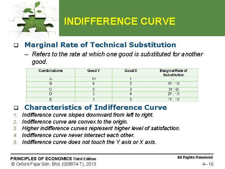
INDIFFERENCE CURVE q Marginal Rate of Technical Substitution – Refers to the rate at which one good is substituted for another good. q 1. 2. 3. 4. 5. Characteristics of Indifference Curve Indifference curve slopes downward from left to right. Indifference curve are convex to the origin. Higher indifference curves represent higher level of satisfaction. Indifference curve never intersect each other. Indifference curve does not touch the Y axis or X axis. PRINCIPLES OF ECONOMICS Third Edition © Oxford Fajar Sdn. Bhd. (008974 -T), 2013 All Rights Reserved 4– 16

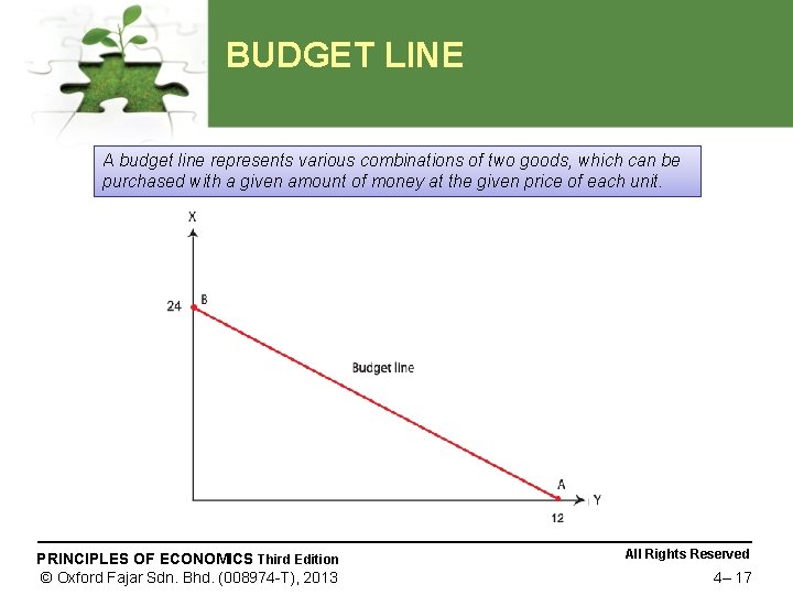
BUDGET LINE A budget line represents various combinations of two goods, which can be purchased with a given amount of money at the given price of each unit. PRINCIPLES OF ECONOMICS Third Edition © Oxford Fajar Sdn. Bhd. (008974 -T), 2013 All Rights Reserved 4– 17

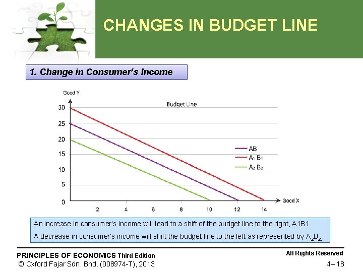
CHANGES IN BUDGET LINE 1. Change in Consumer’s Income An increase in consumer’s income will lead to a shift of the budget line to the right, A 1 B 1. A decrease in consumer’s income will shift the budget line to the left as represented by A 2 B 2. PRINCIPLES OF ECONOMICS Third Edition © Oxford Fajar Sdn. Bhd. (008974 -T), 2013 All Rights Reserved 4– 18

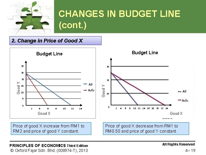
CHANGES IN BUDGET LINE (cont. ) 2. Change in Price of Good X Budget Line 30 30 25 20 AB 15 A 1 B 1 10 5 0 Good Y 20 AB 10 A 1 B 1 2 4 6 8 10 12 14 Good X 0 2 4 6 8 10 12 14 16 18 20 22 24 Good X Price of good X increase from RM 1 to RM 2 and price of good Y constant. PRINCIPLES OF ECONOMICS Third Edition © Oxford Fajar Sdn. Bhd. (008974 -T), 2013 Price of good X decrease from RM 1 to RM 0. 50 and price of good Y constant. All Rights Reserved 4– 19

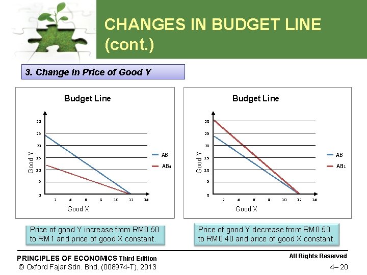
CHANGES IN BUDGET LINE (cont. ) 3. Change in Price of Good Y Budget Line 30 30 25 25 20 20 AB 15 AB 1 10 5 0 Good Y Budget Line AB 15 AB 1 10 5 2 4 6 8 10 12 14 Good X Price of good Y increase from RM 0. 50 to RM 1 and price of good X constant. PRINCIPLES OF ECONOMICS Third Edition © Oxford Fajar Sdn. Bhd. (008974 -T), 2013 0 2 4 6 8 10 12 14 Good X Price of good Y decrease from RM 0. 50 to RM 0. 40 and price of good X constant. All Rights Reserved 4– 20

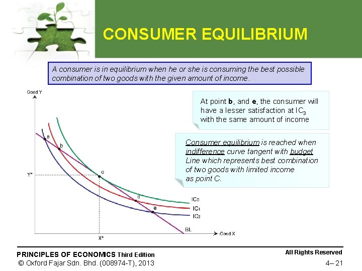
CONSUMER EQUILIBRIUM A consumer is in equilibrium when he or she is consuming the best possible combination of two goods with the given amount of income. At point b, and e, the consumer will have a lesser satisfaction at IC 3 with the same amount of income Consumer equilibrium is reached when indifference curve tangent with budget Line which represents best combination of two goods with limited income as point C. PRINCIPLES OF ECONOMICS Third Edition © Oxford Fajar Sdn. Bhd. (008974 -T), 2013 All Rights Reserved 4– 21

INCOME, PRICE AND SUBSTITUTION EFFECT q INCOME EFFECT – The income effect is defined as the effect on the purchases of the consumer caused by changes in income with prices of goods remaining constant. q PRICE EFFECT – Price effect explains what happens to the consumers’ equilibrium position when the price of one good changes while the price of another good and other factors remains constant. q SUBSTITUTION EFFECT – Substitution effect explains what happens to the consumers’ equilibrium position when the price of both good changes—price of one rises and price of another falls while other factors remains constant. PRINCIPLES OF ECONOMICS Third Edition © Oxford Fajar Sdn. Bhd. (008974 -T), 2013 All Rights Reserved 4– 22

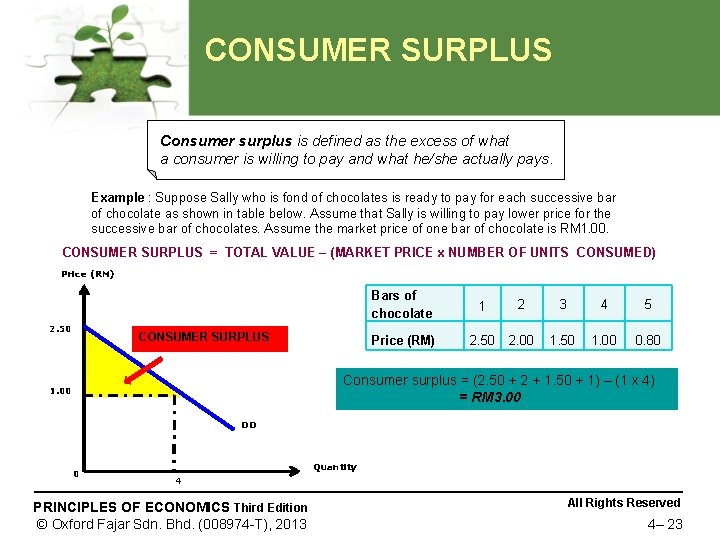
CONSUMER SURPLUS Consumer surplus is defined as the excess of what a consumer is willing to pay and what he/she actually pays. Example : Suppose Sally who is fond of chocolates is ready to pay for each successive bar of chocolate as shown in table below. Assume that Sally is willing to pay lower price for the successive bar of chocolates. Assume the market price of one bar of chocolate is RM 1. 00. CONSUMER SURPLUS = TOTAL VALUE – (MARKET PRICE x NUMBER OF UNITS CONSUMED) Price (RM) 2. 50 CONSUMER SURPLUS Bars of chocolate 1 2 3 4 5 Price (RM) 2. 50 2. 00 1. 50 1. 00 0. 80 Consumer surplus = (2. 50 + 2 + 1. 50 + 1) – (1 x 4) = RM 3. 00 1. 00 DD 0 Quantity 4 PRINCIPLES OF ECONOMICS Third Edition © Oxford Fajar Sdn. Bhd. (008974 -T), 2013 All Rights Reserved 4– 23