PRINCIPLES OF ECONOMICS Third Edition Oxford Fajar Sdn

PRINCIPLES OF ECONOMICS Third Edition © Oxford Fajar Sdn. Bhd. (008974 -T), 2013 All Rights Reserved 7– 1

CHAPTER 7 MARKET STRUCTURE 1: PERFECT COMPETITION AND MONOPOLY PRINCIPLES OF ECONOMICS Third Edition © Oxford Fajar Sdn. Bhd. (008974 -T), 2013 All Rights Reserved 7– 2

DEFINITION AND OBJECTIVES OF A FIRM q Definition of a Firm – A firm is an institution that buys or hires factors of production and organizes them to produce and sell goods and services. – A firm is an independent unit of producing goods and services for sale. q Objectives of a Firm – The main goal or objective of a firm is to maximize profit and to minimize the cost. PRINCIPLES OF ECONOMICS Third Edition © Oxford Fajar Sdn. Bhd. (008974 -T), 2013 All Rights Reserved 7– 3

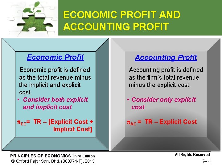
ECONOMIC PROFIT AND ACCOUNTING PROFIT Economic Profit Accounting Profit Economic profit is defined as the total revenue minus the implicit and explicit cost. • Consider both explicit and implicit cost Accounting profit is defined as the firm’s total revenue minus the explicit cost. EC= TR – [Explicit Cost + Implicit Cost] AC = TR – Explicit Cost PRINCIPLES OF ECONOMICS Third Edition © Oxford Fajar Sdn. Bhd. (008974 -T), 2013 • Consider only explicit cost All Rights Reserved 7– 4

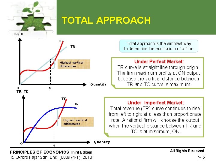
TOTAL APPROACH TR, TC TC Total approach is the simplest way to determine the equilibrium of a firm. TR Under Perfect Market: TR curve is straight line through origin. The firm maximum profits at ON output because the vertical distance between TR and TC curve is maximum. Highest vertical differences 0 TR, TC Quantity N TC TR Highest vertical differences O N PRINCIPLES OF ECONOMICS Third Edition © Oxford Fajar Sdn. Bhd. (008974 -T), 2013 Under Imperfect Market: Total revenue (TR) curve continues to rise from left to right at a less than proportionate rate. A rational firm will choose the output when the vertical distance between TR and TC is at maximum, ON. Quantity All Rights Reserved 7– 5

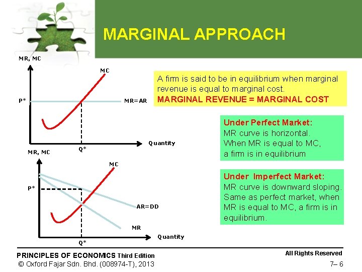
MARGINAL APPROACH MR, MC MC P* A firm is said to be in equilibrium when marginal revenue is equal to marginal cost. MARGINAL REVENUE = MARGINAL COST MR=AR MR, MC Quantity Q* Under Perfect Market: MR curve is horizontal. When MR is equal to MC, a firm is in equilibrium MC P* AR=DD Under Imperfect Market: MR curve is downward sloping. Same as perfect market, when MR is equal to MC, a firm is in equilibrium. MR Q* PRINCIPLES OF ECONOMICS Third Edition © Oxford Fajar Sdn. Bhd. (008974 -T), 2013 Quantity All Rights Reserved 7– 6

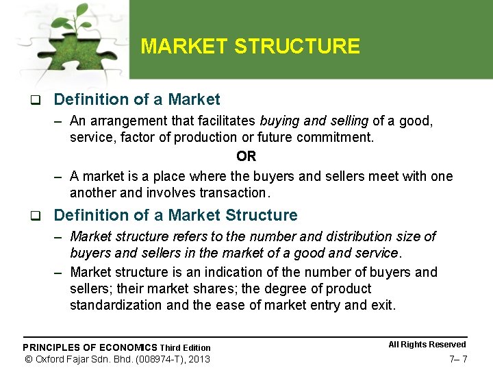
MARKET STRUCTURE q Definition of a Market – An arrangement that facilitates buying and selling of a good, service, factor of production or future commitment. OR – A market is a place where the buyers and sellers meet with one another and involves transaction. q Definition of a Market Structure – Market structure refers to the number and distribution size of buyers and sellers in the market of a good and service. – Market structure is an indication of the number of buyers and sellers; their market shares; the degree of product standardization and the ease of market entry and exit. PRINCIPLES OF ECONOMICS Third Edition © Oxford Fajar Sdn. Bhd. (008974 -T), 2013 All Rights Reserved 7– 7

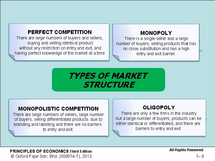
PERFECT COMPETITION There are large numbers of buyers and sellers, buying and selling identical product without any restriction on entry and exit, and having perfect knowledge of the market at a time. MONOPOLY There is a single seller and a large number of buyers; selling products that has no close substitution and has a high entry and exit barrier. TYPES OF MARKET STRUCTURE MONOPOLISTIC COMPETITION There are large numbers of sellers, large number of buyers; selling differentiated products due to branding and labelling and there are no barriers to entry and exit. PRINCIPLES OF ECONOMICS Third Edition © Oxford Fajar Sdn. Bhd. (008974 -T), 2013 OLIGOPOLY There are only a few firms in the industry but a large number of buyers; products can be either identical or differentiated, and there are barriers to entry and exit. All Rights Reserved 7– 8

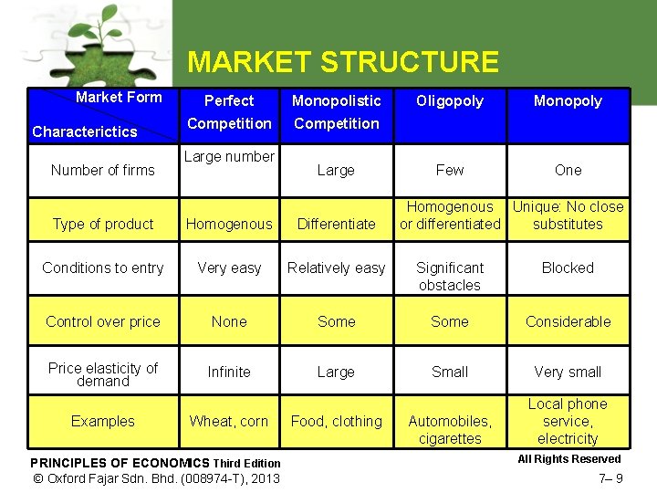
MARKET STRUCTURE Market Form Characterictics Number of firms Perfect Monopolistic Competition Large number Large Oligopoly Monopoly Few One Homogenous Unique: No close or differentiated substitutes Type of product Homogenous Differentiate Conditions to entry Very easy Relatively easy Significant obstacles Blocked Control over price None Some Considerable Infinite Large Small Very small Automobiles, cigarettes Local phone service, electricity Price elasticity of demand Examples Wheat, corn PRINCIPLES OF ECONOMICS Third Edition © Oxford Fajar Sdn. Bhd. (008974 -T), 2013 Food, clothing All Rights Reserved 7– 9

PERFECT COMPETITION q Definition – A market in which there are many buyers and sellers, the products are homogeneous and sellers can easily enter and exit from the market. q Characteristics – Large number of buyers and sellers – firms are price takers – Homogenous or standardized product – the buyers do not differentiate the products of one seller to another seller – Free of entry and exit into the market – Role of non-price competition is insignificant PRINCIPLES OF ECONOMICS Third Edition © Oxford Fajar Sdn. Bhd. (008974 -T), 2013 All Rights Reserved 7– 10

PERFECT COMPETITION (cont. ) – Perfect knowledge of the market – all the sellers and buyers in perfect competition market will have perfect knowledge of that market – Perfect mobility of factor of production – factor of production can freely move from one occupation to another and from one place to another – Absence of transport cost PRINCIPLES OF ECONOMICS Third Edition © Oxford Fajar Sdn. Bhd. (008974 -T), 2013 All Rights Reserved 7– 11

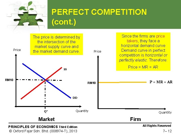
PERFECT COMPETITION (cont. ) Price The price is determined by the intersection of the market supply curve and the market demand curve. Price Since the firms are price takers, they face a horizontal demand curve Demand curve in perfect competition is horizontal or perfectly elastic. Therefore: Price = MR = AR SS RM 10 P = MR = AR RM 10 DD Q* Quantity Market PRINCIPLES OF ECONOMICS Third Edition © Oxford Fajar Sdn. Bhd. (008974 -T), 2013 Quantity Firm All Rights Reserved 7– 12

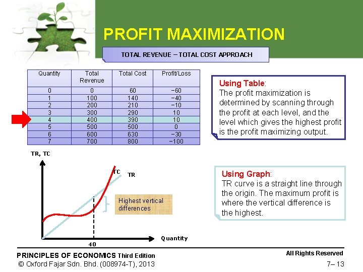
PROFIT MAXIMIZATION TOTAL REVENUE – TOTAL COST APPROACH Quantity 0 1 2 3 4 5 6 7 Total Revenue Total Cost 0 100 200 300 400 500 600 700 60 140 210 290 390 500 630 800 Profit/Loss − 60 − 40 − 10 10 10 0 − 30 − 100 Using Table: The profit maximization is determined by scanning through the profit at each level, and the level which gives the highest profit is the profit maximizing output. TR, TC TC TR Highest vertical differences 40 PRINCIPLES OF ECONOMICS Third Edition © Oxford Fajar Sdn. Bhd. (008974 -T), 2013 Using Graph: TR curve is a straight line through the origin. The maximum profit is where the vertical difference is the highest. Quantity All Rights Reserved 7– 13

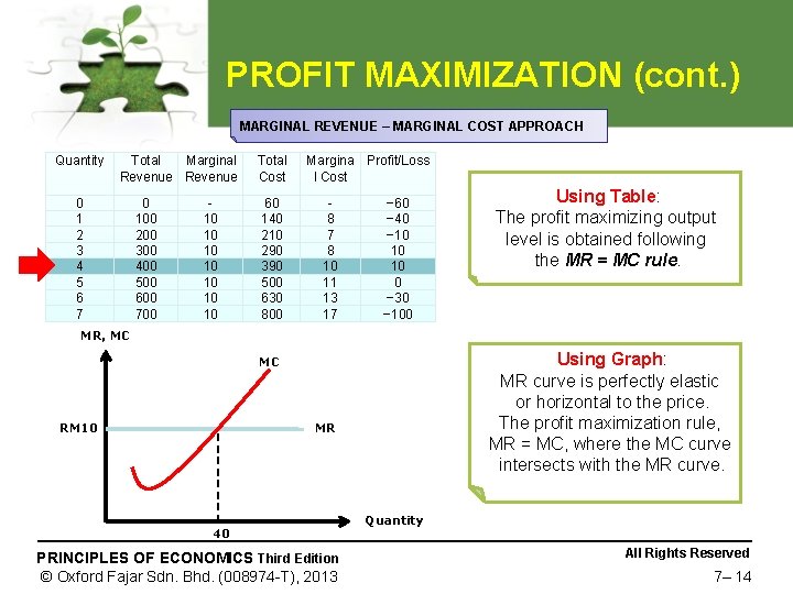
PROFIT MAXIMIZATION (cont. ) MARGINAL REVENUE – MARGINAL COST APPROACH Quantity Total Marginal Revenue 0 1 2 3 4 5 6 7 0 100 200 300 400 500 600 700 10 10 Total Cost 60 140 210 290 390 500 630 800 Margina Profit/Loss l Cost 8 7 8 10 11 13 17 − 60 − 40 − 10 10 10 0 − 30 − 100 Using Table: The profit maximizing output level is obtained following the MR = MC rule. MR, MC Using Graph: MR curve is perfectly elastic or horizontal to the price. The profit maximization rule, MR = MC, where the MC curve intersects with the MR curve. MC RM 10 MR 40 PRINCIPLES OF ECONOMICS Third Edition © Oxford Fajar Sdn. Bhd. (008974 -T), 2013 Quantity All Rights Reserved 7– 14

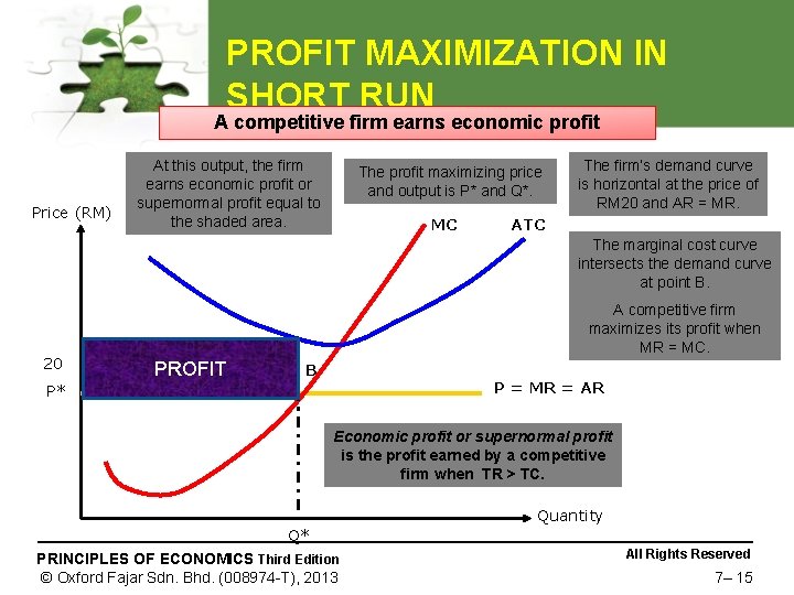
PROFIT MAXIMIZATION IN SHORT RUN A competitive firm earns economic profit Price (RM) At this output, the firm earns economic profit or supernormal profit equal to the shaded area. The profit maximizing price and output is P* and Q*. MC The firm’s demand curve is horizontal at the price of RM 20 and AR = MR. ATC The marginal cost curve intersects the demand curve at point B. 20 A competitive firm maximizes its profit when MR = MC. PROFIT B P = MR = AR P* Economic profit or supernormal profit is the profit earned by a competitive firm when TR > TC. Quantity Q* PRINCIPLES OF ECONOMICS Third Edition © Oxford Fajar Sdn. Bhd. (008974 -T), 2013 All Rights Reserved 7– 15

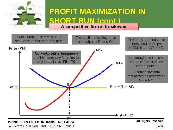
PROFIT MAXIMIZATION IN SHORT RUN (cont. ) A competitive firm at breakeven At this output, the firm is at the breakeven or earns normal profit. The profit maximizing price and output is P* and Q*. Price (RM) Normal profit or breakeven profit is necessary for a firm to stay in business TR = TC The firm’s demand curve is horizontal at the price of RM 20 and AR = MR. MC ATC The marginal cost curve intersects the demand curve at point B. A competitive firm maximizes its profit when MR = MC. P* 20 B Q* PRINCIPLES OF ECONOMICS Third Edition © Oxford Fajar Sdn. Bhd. (008974 -T), 2013 P = MR = AR Quantity All Rights Reserved 7– 16

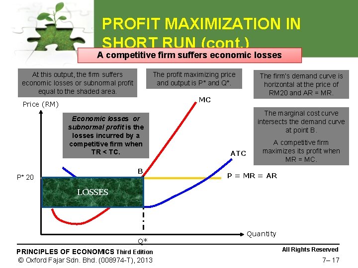
PROFIT MAXIMIZATION IN SHORT RUN (cont. ) A competitive firm suffers economic losses At this output, the firm suffers economic losses or subnormal profit equal to the shaded area. The profit maximizing price and output is P* and Q*. MC Price (RM) Economic losses or subnormal profit is the losses incurred by a competitive firm when TR < TC. B P* 20 The firm’s demand curve is horizontal at the price of RM 20 and AR = MR. The marginal cost curve intersects the demand curve at point B. ATC A competitive firm maximizes its profit when MR = MC. P = MR = AR LOSSES Q* PRINCIPLES OF ECONOMICS Third Edition © Oxford Fajar Sdn. Bhd. (008974 -T), 2013 Quantity All Rights Reserved 7– 17

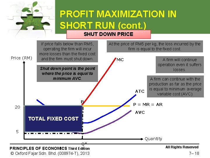
PROFIT MAXIMIZATION IN SHORT RUN (cont. ) SHUT DOWN PRICE Price (RM) If price falls below than RM 5, operating the firm will incur more losses than the fixed cost and the firm must shut down. At the price of RM 5 per kg, the loss incurred by the firm is equal to the fixed cost. MC A firm will continue operation even it suffers losses. Shut down point is the point where the price is equal to minimum AVC. ATC B 20 A firm can continue with the production as far as the price is equal to minimum average variable cost (AVC). P = MR = AR AVC LOSSES TOTAL FIXED COST 5 Quantity Q* PRINCIPLES OF ECONOMICS Third Edition © Oxford Fajar Sdn. Bhd. (008974 -T), 2013 All Rights Reserved 7– 18

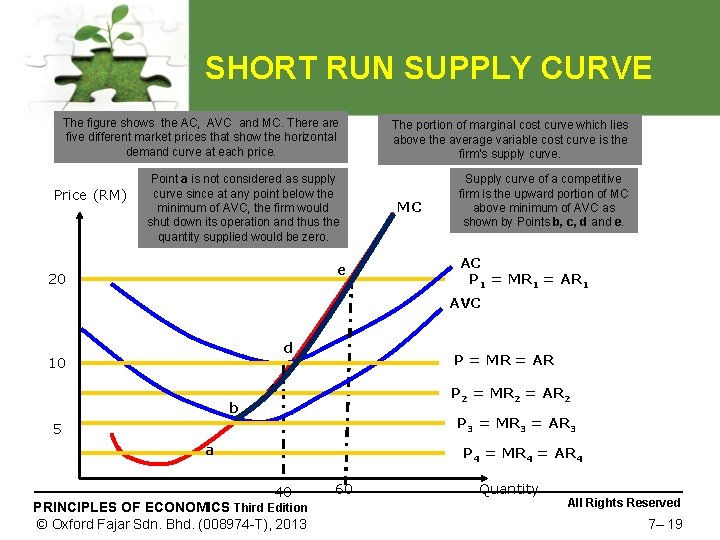
SHORT RUN SUPPLY CURVE The figure shows the AC, AVC and MC. There are five different market prices that show the horizontal demand curve at each price. The portion of marginal cost curve which lies above the average variable cost curve is the firm’s supply curve. Point a is not considered as supply curve since at any point below the minimum of AVC, the firm would shut down its operation and thus the quantity supplied would be zero. Supply curve of a competitive firm is the upward portion of MC above minimum of AVC as shown by Points b, c, d and e. Price (RM) e 20 MC AC P 1 = MR 1 = AR 1 AVC d 10 P = MR = AR c P 2 = MR 2 = AR 2 b P 3 = MR 3 = AR 3 5 a P 4 = MR 4 = AR 4 40 PRINCIPLES OF ECONOMICS Third Edition © Oxford Fajar Sdn. Bhd. (008974 -T), 2013 60 Quantity All Rights Reserved 7– 19

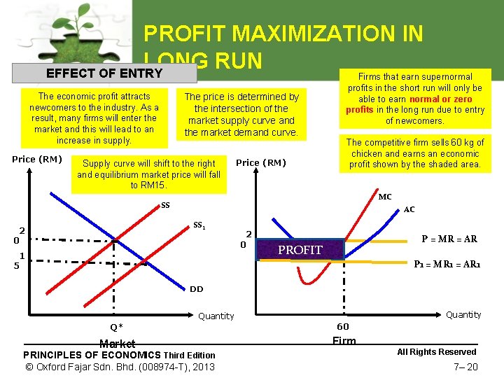
PROFIT MAXIMIZATION IN LONG RUN EFFECT OF ENTRY The economic profit attracts newcomers to the industry. As a result, many firms will enter the market and this will lead to an increase in supply. Price (RM) The price is determined by the intersection of the market supply curve and the market demand curve. Supply curve will shift to the right and equilibrium market price will fall to RM 15. Price (RM) Firms that earn supernormal profits in the short run will only be able to earn normal or zero profits in the long run due to entry of newcomers. The competitive firm sells 60 kg of chicken and earns an economic profit shown by the shaded area. MC SS AC SS 1 2 0 1 5 2 0 P = MR = AR PROFIT P 1 = MR 1 = AR 1 DD Quantity Q* 60 Market Firm PRINCIPLES OF ECONOMICS Third Edition © Oxford Fajar Sdn. Bhd. (008974 -T), 2013 All Rights Reserved 7– 20

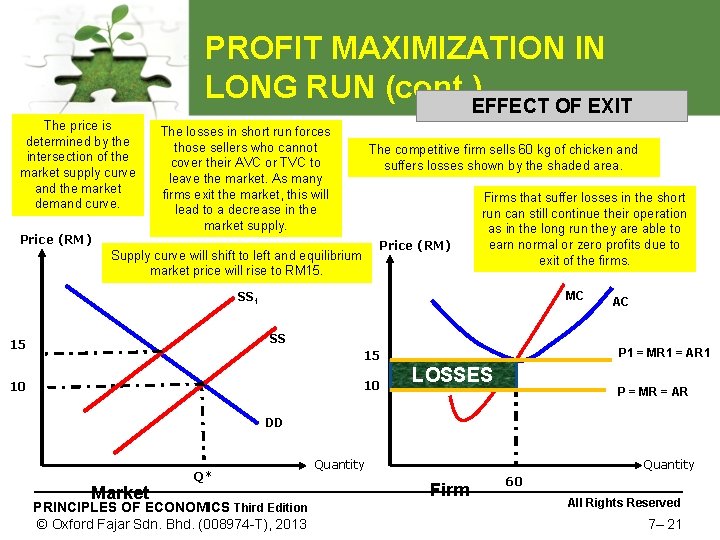
PROFIT MAXIMIZATION IN LONG RUN (cont. )EFFECT OF EXIT The price is determined by the intersection of the market supply curve and the market demand curve. Price (RM) The losses in short run forces those sellers who cannot cover their AVC or TVC to leave the market. As many firms exit the market, this will lead to a decrease in the market supply. The competitive firm sells 60 kg of chicken and suffers losses shown by the shaded area. Supply curve will shift to left and equilibrium market price will rise to RM 15. Price (RM) Firms that suffer losses in the short run can still continue their operation as in the long run they are able to earn normal or zero profits due to exit of the firms. MC SS 1 AC SS 15 P 1 = MR 1 = AR 1 15 10 10 LOSSES P = MR = AR DD Market Q* PRINCIPLES OF ECONOMICS Third Edition © Oxford Fajar Sdn. Bhd. (008974 -T), 2013 Quantity Firm 60 All Rights Reserved 7– 21

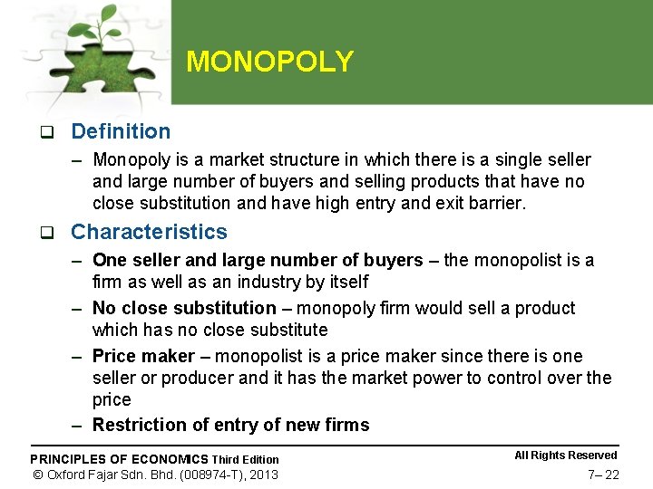
MONOPOLY q Definition – Monopoly is a market structure in which there is a single seller and large number of buyers and selling products that have no close substitution and have high entry and exit barrier. q Characteristics – One seller and large number of buyers – the monopolist is a firm as well as an industry by itself – No close substitution – monopoly firm would sell a product which has no close substitute – Price maker – monopolist is a price maker since there is one seller or producer and it has the market power to control over the price – Restriction of entry of new firms PRINCIPLES OF ECONOMICS Third Edition © Oxford Fajar Sdn. Bhd. (008974 -T), 2013 All Rights Reserved 7– 22

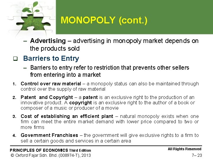
MONOPOLY (cont. ) – Advertising – advertising in monopoly market depends on the products sold q Barriers to Entry – Barriers to entry refer to restriction that prevents other sellers from entering into a market 1. Control over raw material – a monopoly status can also be maintained through control over the supply of raw material 2. Patent and Copyright – a patent is an exclusive right to the production of an innovative product. A copyright is an exclusive right to the author of a book or composer of a music or producer of a movie 3. Cost of establishing an efficient plant – natural monopoly exists when one firm can meet the entire market demand with lower price compared to two or more firms 4. Government Franchises – the government will give exclusive rights to a firm to sell a certain goods and services in a certain area PRINCIPLES OF ECONOMICS Third Edition © Oxford Fajar Sdn. Bhd. (008974 -T), 2013 All Rights Reserved 7– 23

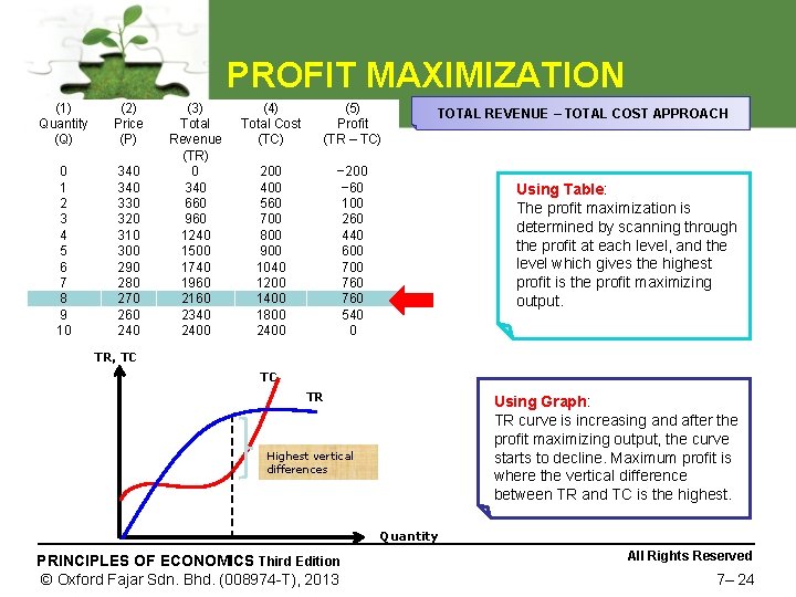
PROFIT MAXIMIZATION (1) Quantity (Q) (2) Price (P) 0 1 2 3 4 5 6 7 8 9 10 340 330 320 310 300 290 280 270 260 240 (3) Total Revenue (TR) 0 340 660 960 1240 1500 1740 1960 2160 2340 2400 (4) Total Cost (TC) (5) Profit (TR – TC) 200 400 560 700 800 900 1040 1200 1400 1800 2400 − 200 − 60 100 260 440 600 760 760 540 0 TOTAL REVENUE – TOTAL COST APPROACH Using Table: The profit maximization is determined by scanning through the profit at each level, and the level which gives the highest profit is the profit maximizing output. TR, TC TC TR Using Graph: TR curve is increasing and after the profit maximizing output, the curve starts to decline. Maximum profit is where the vertical difference between TR and TC is the highest. Highest vertical differences Quantity PRINCIPLES OF ECONOMICS Third Edition © Oxford Fajar Sdn. Bhd. (008974 -T), 2013 All Rights Reserved 7– 24

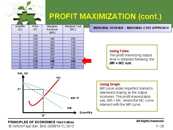
PROFIT MAXIMIZATION (cont. ) Quantity (Q) Price (P) 0 1 2 3 4 5 6 7 8 9 10 340 330 320 310 300 290 280 270 260 240 Marginal Revenue (MR) Marginal Cost (MC) 340 320 300 280 260 240 220 200 180 60 200 160 140 100 140 160 200 400 600 MARGINAL REVENUE – MARGINAL COST APPROACH Using Table: The profit maximizing output level is obtained following the MR = MC rule. MR, MC MC Using Graph: MR curve under imperfect market is downward sloping as the output increases. The profit maximization rule, MR = MC, where the MC curve intersect with the MR curve. P* AR=P MR Q* PRINCIPLES OF ECONOMICS Third Edition © Oxford Fajar Sdn. Bhd. (008974 -T), 2013 Quantity All Rights Reserved 7– 25

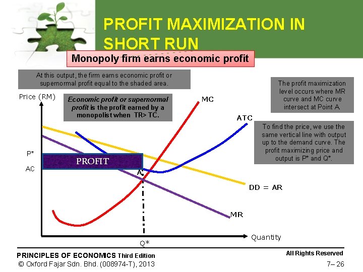
PROFIT MAXIMIZATION IN SHORT RUN Monopoly firm earns economic profit At this output, the firm earns economic profit or supernormal profit equal to the shaded area. Price (RM) P* AC Economic profit or supernormal profit is the profit earned by a monopolist when TR> TC. The profit maximization level occurs where MR curve and MC curve intersect at Point A. MC ATC To find the price, we use the same vertical line with output up to the demand curve. The profit maximizing price and output is P* and Q*. PROFIT A DD = AR MR Q* PRINCIPLES OF ECONOMICS Third Edition © Oxford Fajar Sdn. Bhd. (008974 -T), 2013 Quantity All Rights Reserved 7– 26

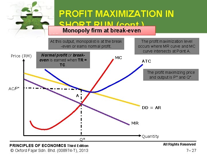
PROFIT MAXIMIZATION IN SHORT RUN (cont. ) Monopoly firm at break-even At this output, monopolist is at the break -even or earns normal profit. Price (RM) Normal profit or breakeven is earned when TR = TC. The profit maximization level occurs where MR curve and MC curve intersects at Point A. MC ATC The profit maximizing price and output is P* and Q*. AC/P* A DD = AR MR Q* PRINCIPLES OF ECONOMICS Third Edition © Oxford Fajar Sdn. Bhd. (008974 -T), 2013 Quantity All Rights Reserved 7– 27

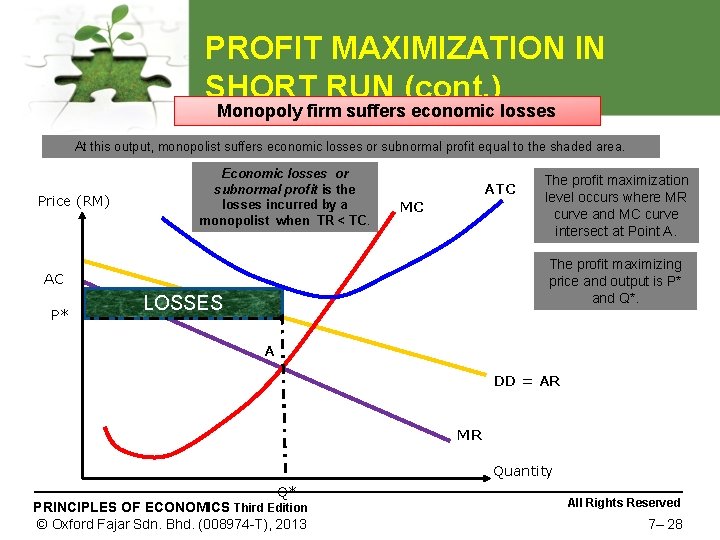
PROFIT MAXIMIZATION IN SHORT RUN (cont. ) Monopoly firm suffers economic losses At this output, monopolist suffers economic losses or subnormal profit equal to the shaded area. Price (RM) Economic losses or subnormal profit is the losses incurred by a monopolist when TR < TC. ATC MC The profit maximizing price and output is P* and Q*. AC P* The profit maximization level occurs where MR curve and MC curve intersect at Point A. LOSSES A DD = AR MR Quantity Q* PRINCIPLES OF ECONOMICS Third Edition © Oxford Fajar Sdn. Bhd. (008974 -T), 2013 All Rights Reserved 7– 28

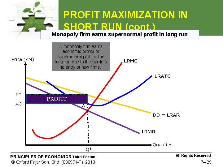
PROFIT MAXIMIZATION IN SHORT RUN (cont. ) Monopoly firm earns supernormal profit in long run Price (RM) A monopoly firm earns economic profits or supernormal profit in the long run due to the barriers to entry of new firms. LRMC LRATC P* AC PROFIT A DD = LRAR LRMR Q* PRINCIPLES OF ECONOMICS Third Edition © Oxford Fajar Sdn. Bhd. (008974 -T), 2013 Quantity All Rights Reserved 7– 29

PRICE DISCRIMINATION Definition – Price discrimination refers to the selling or charging of different prices by a firm to different buyers for the same product. q Necessary Conditions – Existence of monopoly power – price discrimination can occur only if monopoly power exists and there are no competitors in the market – Existence of different markets for the same commodity – a firm should be able to separate customers according to price elasticity of demand q PRINCIPLES OF ECONOMICS Third Edition © Oxford Fajar Sdn. Bhd. (008974 -T), 2013 All Rights Reserved 7– 30

PRICE DISCRIMINATION (cont. ) – Existence of different degree of elasticity of demand – monopolist can charge higher price for inelastic market and lower price for elastic market – Cost of separating market must be low – No resale – product purchased in the low-priced market should not be resold in the high-priced market – Legal sanction – government allows the public utility firms such as electricity to charge different prices from different consumers PRINCIPLES OF ECONOMICS Third Edition © Oxford Fajar Sdn. Bhd. (008974 -T), 2013 All Rights Reserved 7– 31

PRICE DISCRIMINATION (cont. ) q First-degree Price Discrimination – Occurs when a firm charges each consumer the maximum price that he or she is willing to pay for each unit. – This price discrimination is also known as perfect price discrimination. – The best example for first-degree price discrimination is auction. q Second-degree Price Discrimination – Occurs when the products are grouped into blocks and each block is charged at a different price. – This type of price discrimination is charged by public utilities such as electricity charges, water charges, telephone charges and others. PRINCIPLES OF ECONOMICS Third Edition © Oxford Fajar Sdn. Bhd. (008974 -T), 2013 All Rights Reserved 7– 32

PRICE DISCRIMINATION (cont. ) q Third-Degree Price Discrimination – Under this price discrimination, the markets are divided into many submarkets or subgroups. – Each group is considered as a different market. – The price charged on products depends on the price elasticity of demand. – An example of third-degree price discrimination is the movie ticket where the adults are charged higher price and children are charged at lower price. – Other examples are transportation (air, railways, bus or LRT), medical, legal and entertainment. PRINCIPLES OF ECONOMICS Third Edition © Oxford Fajar Sdn. Bhd. (008974 -T), 2013 All Rights Reserved 7– 33

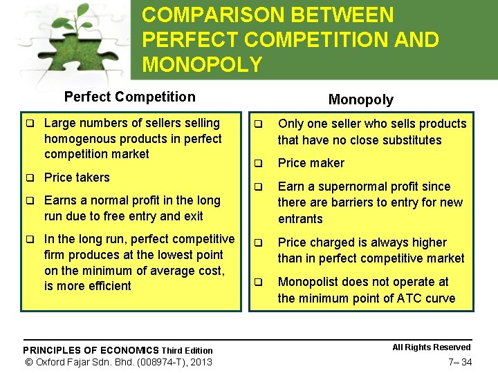
COMPARISON BETWEEN PERFECT COMPETITION AND MONOPOLY Perfect Competition q Large numbers of sellers selling homogenous products in perfect competition market q Price takers q Earns a normal profit in the long run due to free entry and exit q In the long run, perfect competitive firm produces at the lowest point on the minimum of average cost, is more efficient PRINCIPLES OF ECONOMICS Third Edition © Oxford Fajar Sdn. Bhd. (008974 -T), 2013 Monopoly q Only one seller who sells products that have no close substitutes q Price maker q Earn a supernormal profit since there are barriers to entry for new entrants q Price charged is always higher than in perfect competitive market q Monopolist does not operate at the minimum point of ATC curve All Rights Reserved 7– 34