Principles of 2 D Image Analysis Part 3

Principles of 2 D Image Analysis Part 3 of 3 Notes prepared by Dr. Bartek Rajwa, Prof. John Turek & Prof. J. Paul Robinson These slides are intended for use in a lecture series. Copies of the graphics are distributed and students encouraged to take their notes on these graphics. The intent is to have the student NOT try to reproduce the figures, but to LISTEN and UNDERSTAND the material. All material copyright J. Paul Robinson unless otherwise stated, however, the material may be freely used for lectures, tutorials and workshops. It may not be used for any commercial purpose. It is illegal to upload this lecture to Course. Hero or any other site. www. cyto. purdue. edu UPDATED Jan 2020 14: 34 © 1997 -2020 J. Turek, B. Rajwa & J. Paul Robinson, Purdue University

Image Processing in the Spatial Domain • Arithmetic and logic operations • Basic gray level transformations on histograms • Spatial filtering • Overview of analytical techniques 14: 34 © 1997 -2020 J. Turek, B. Rajwa & J. Paul Robinson, Purdue University

Modifying image contrast and brightness • The easiest and most frequent method is histogram manipulation • An 8 bit gray scale image will display 28 =256 different brightness levels ranging from 0 (black) to 255 (white) (210=1024, 212=4096). An image that has pixel values throughout the entire range has a large dynamic range, and may or may not display the appropriate contrast for the features of interest. 16 bit would be 216 (or 65, 536) • (Non-linear enhancements - e. g. Equalization see later) 14: 34 © 1997 -2020 J. Turek, B. Rajwa & J. Paul Robinson, Purdue University

Image Processing. . is the procedure of feature enhancement prior to image analysis. Image processing is performed on pixels (smallest unit of digital image data). The various algorithms used in image processing and morphological analysis perform their operations on groups of pixels (3 X 3, 5 X 5, etc. ) called kernels. These image processing kernels may also be used as structuring elements for the various image morphological analysis operations. 14: 34 © 1997 -2020 J. Turek, B. Rajwa & J. Paul Robinson, Purdue University

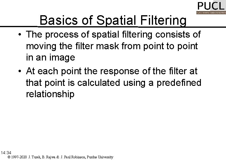
Basics of Spatial Filtering • The process of spatial filtering consists of moving the filter mask from point to point in an image • At each point the response of the filter at that point is calculated using a predefined relationship 14: 34 © 1997 -2020 J. Turek, B. Rajwa & J. Paul Robinson, Purdue University

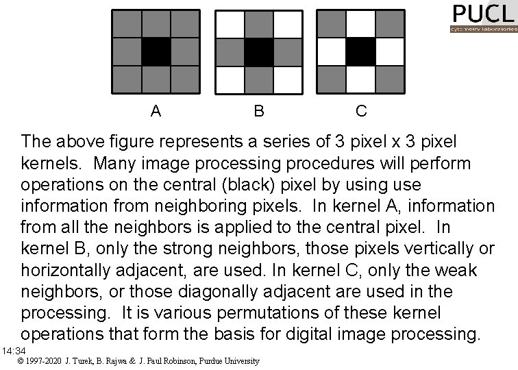
A B C The above figure represents a series of 3 pixel x 3 pixel kernels. Many image processing procedures will perform operations on the central (black) pixel by using use information from neighboring pixels. In kernel A, information from all the neighbors is applied to the central pixel. In kernel B, only the strong neighbors, those pixels vertically or horizontally adjacent, are used. In kernel C, only the weak neighbors, or those diagonally adjacent are used in the processing. It is various permutations of these kernel operations that form the basis for digital image processing. 14: 34 © 1997 -2020 J. Turek, B. Rajwa & J. Paul Robinson, Purdue University

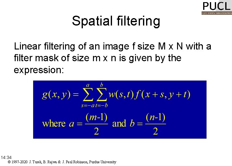
Spatial filtering Linear filtering of an image f size M x N with a filter mask of size m x n is given by the expression: 14: 34 © 1997 -2020 J. Turek, B. Rajwa & J. Paul Robinson, Purdue University

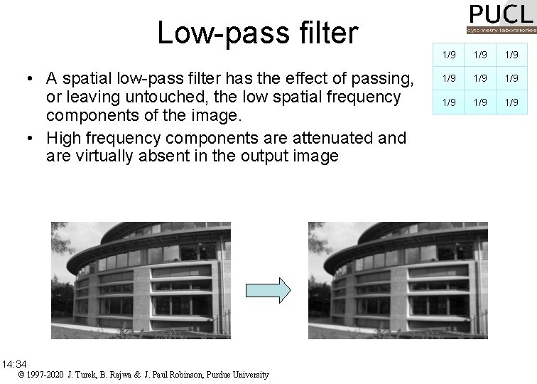
Low-pass filter • A spatial low-pass filter has the effect of passing, or leaving untouched, the low spatial frequency components of the image. • High frequency components are attenuated and are virtually absent in the output image 14: 34 © 1997 -2020 J. Turek, B. Rajwa & J. Paul Robinson, Purdue University 1/9 1/9 1/9

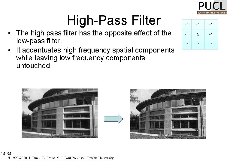
High-Pass Filter • The high pass filter has the opposite effect of the low-pass filter. • It accentuates high frequency spatial components while leaving low frequency components untouched 14: 34 © 1997 -2020 J. Turek, B. Rajwa & J. Paul Robinson, Purdue University -1 -1 9 -1 -1

Edge Detection and Enhancement • Image edge enhancement reduces an image to show only its edges. • Edge enhancements are based on the pixel brightness slope occurring within a group of pixel 14: 34 © 1997 -2020 J. Turek, B. Rajwa & J. Paul Robinson, Purdue University

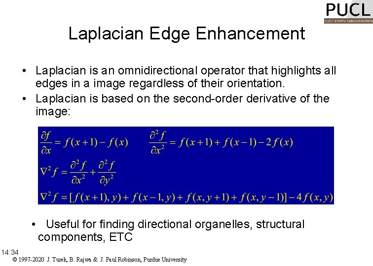
Laplacian Edge Enhancement • Laplacian is an omnidirectional operator that highlights all edges in a image regardless of their orientation. • Laplacian is based on the second-order derivative of the image: • Useful for finding directional organelles, structural components, ETC 14: 34 © 1997 -2020 J. Turek, B. Rajwa & J. Paul Robinson, Purdue University

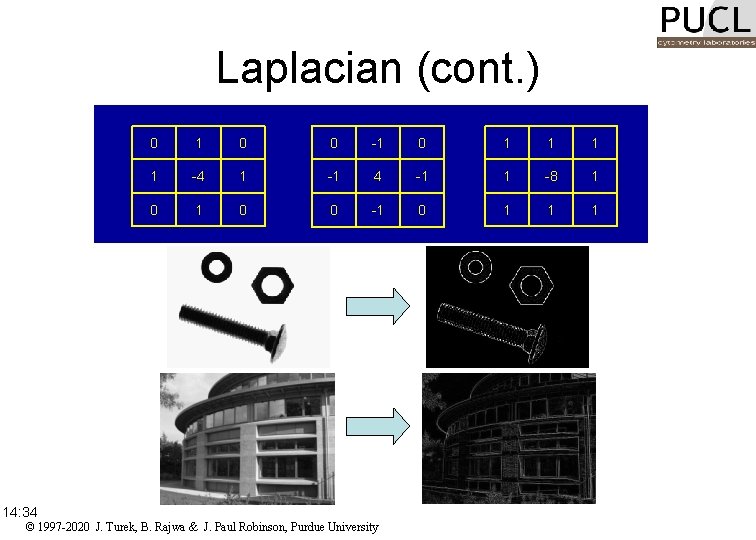
Laplacian (cont. ) 14: 34 0 1 0 0 -1 0 1 1 -4 1 -1 4 -1 1 -8 1 0 0 -1 0 1 1 1 © 1997 -2020 J. Turek, B. Rajwa & J. Paul Robinson, Purdue University

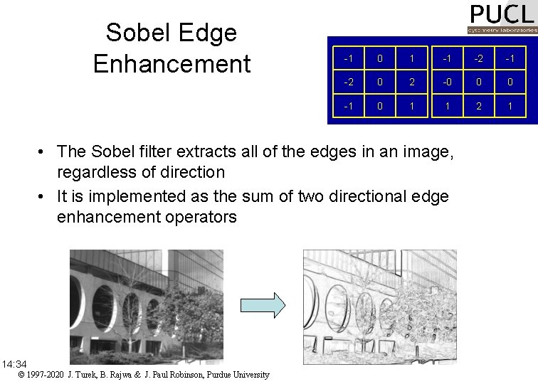
Sobel Edge Enhancement -1 0 1 -1 -2 0 2 -0 0 0 -1 0 1 1 2 1 • The Sobel filter extracts all of the edges in an image, regardless of direction • It is implemented as the sum of two directional edge enhancement operators 14: 34 © 1997 -2020 J. Turek, B. Rajwa & J. Paul Robinson, Purdue University

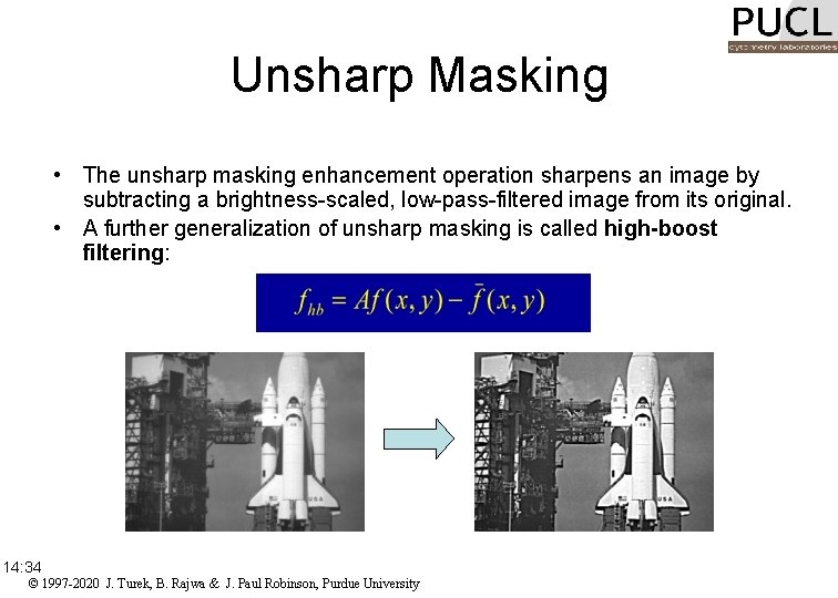
Unsharp Masking • The unsharp masking enhancement operation sharpens an image by subtracting a brightness-scaled, low-pass-filtered image from its original. • A further generalization of unsharp masking is called high-boost filtering: 14: 34 © 1997 -2020 J. Turek, B. Rajwa & J. Paul Robinson, Purdue University

Shape analysis • Shape measurements are physical dimensional measures that characterize the appearance of an object. • The goal is to use the fewest necessary measures to characterize an object adequately so that it may be unambiguously classified. • The shape may not be entirely reconstructable from the descriptors, but the descriptors for different shapes should be different enough that the shapes can be discriminated. 14: 34 © 1997 -2020 J. Turek, B. Rajwa & J. Paul Robinson, Purdue University

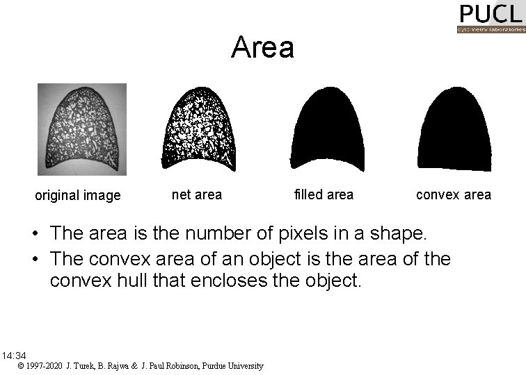
Area original image net area filled area convex area • The area is the number of pixels in a shape. • The convex area of an object is the area of the convex hull that encloses the object. 14: 34 © 1997 -2020 J. Turek, B. Rajwa & J. Paul Robinson, Purdue University

Perimeter perimeter external perimeter convex perimeter • The perimeter [length] is the number of pixels in the boundary of the object. • The convex perimeter of an object is the perimeter of the convex hull that encloses the object. 14: 34 © 1997 -2020 J. Turek, B. Rajwa & J. Paul Robinson, Purdue University

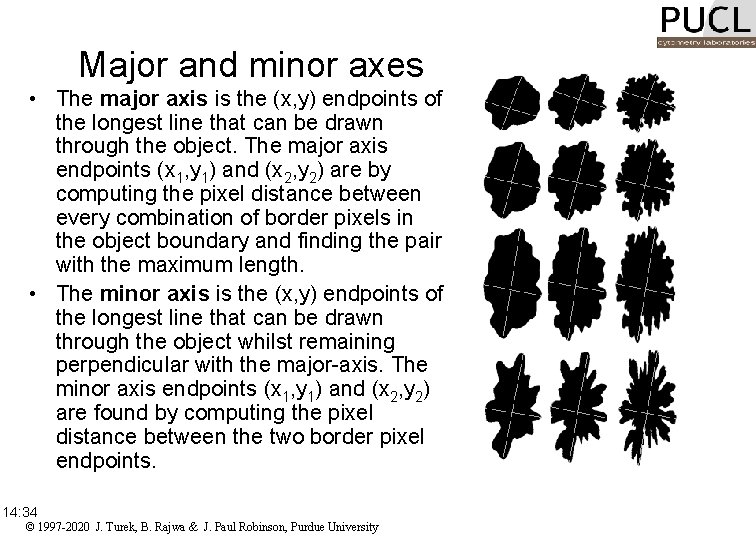
Major and minor axes • The major axis is the (x, y) endpoints of the longest line that can be drawn through the object. The major axis endpoints (x 1, y 1) and (x 2, y 2) are by computing the pixel distance between every combination of border pixels in the object boundary and finding the pair with the maximum length. • The minor axis is the (x, y) endpoints of the longest line that can be drawn through the object whilst remaining perpendicular with the major-axis. The minor axis endpoints (x 1, y 1) and (x 2, y 2) are found by computing the pixel distance between the two border pixel endpoints. 14: 34 © 1997 -2020 J. Turek, B. Rajwa & J. Paul Robinson, Purdue University

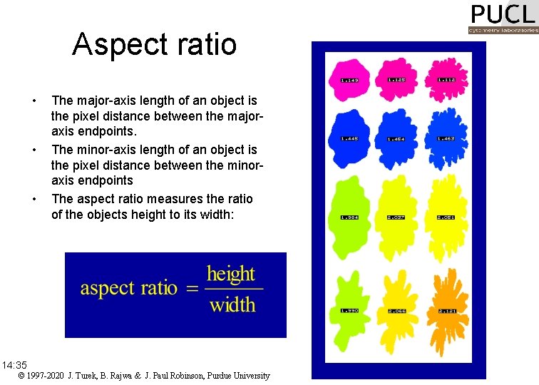
Aspect ratio • • • 14: 35 The major-axis length of an object is the pixel distance between the majoraxis endpoints. The minor-axis length of an object is the pixel distance between the minoraxis endpoints The aspect ratio measures the ratio of the objects height to its width: © 1997 -2020 J. Turek, B. Rajwa & J. Paul Robinson, Purdue University

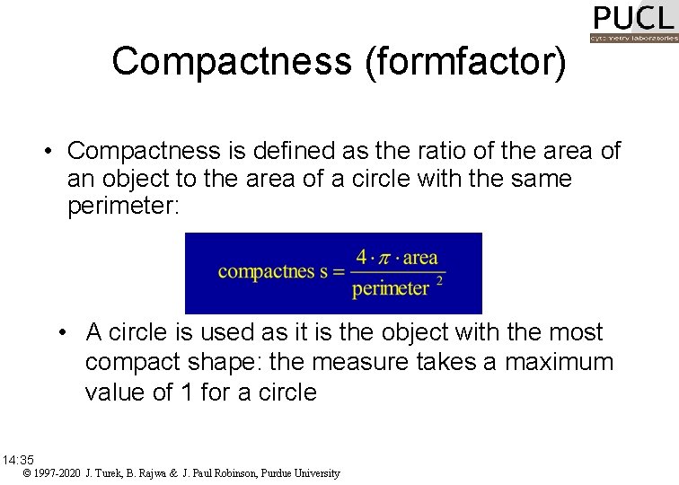
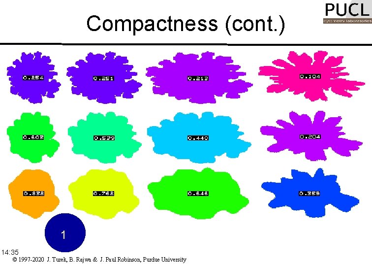
Compactness (formfactor) • Compactness is defined as the ratio of the area of an object to the area of a circle with the same perimeter: • A circle is used as it is the object with the most compact shape: the measure takes a maximum value of 1 for a circle 14: 35 © 1997 -2020 J. Turek, B. Rajwa & J. Paul Robinson, Purdue University

Compactness (cont. ) 1 14: 35 © 1997 -2020 J. Turek, B. Rajwa & J. Paul Robinson, Purdue University

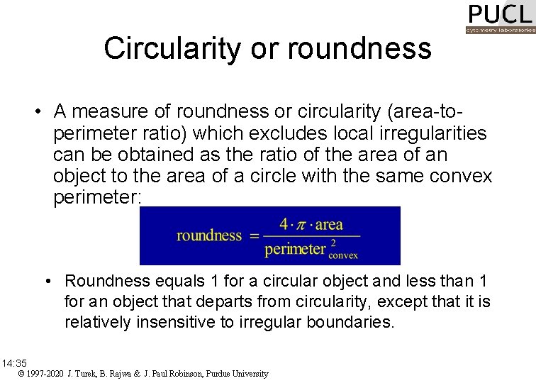
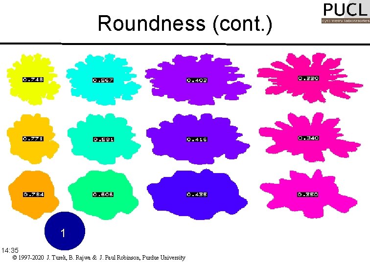
Circularity or roundness • A measure of roundness or circularity (area-toperimeter ratio) which excludes local irregularities can be obtained as the ratio of the area of an object to the area of a circle with the same convex perimeter: • Roundness equals 1 for a circular object and less than 1 for an object that departs from circularity, except that it is relatively insensitive to irregular boundaries. 14: 35 © 1997 -2020 J. Turek, B. Rajwa & J. Paul Robinson, Purdue University

Roundness (cont. ) 1 14: 35 © 1997 -2020 J. Turek, B. Rajwa & J. Paul Robinson, Purdue University

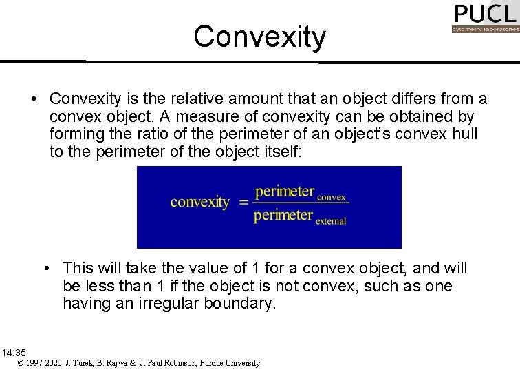
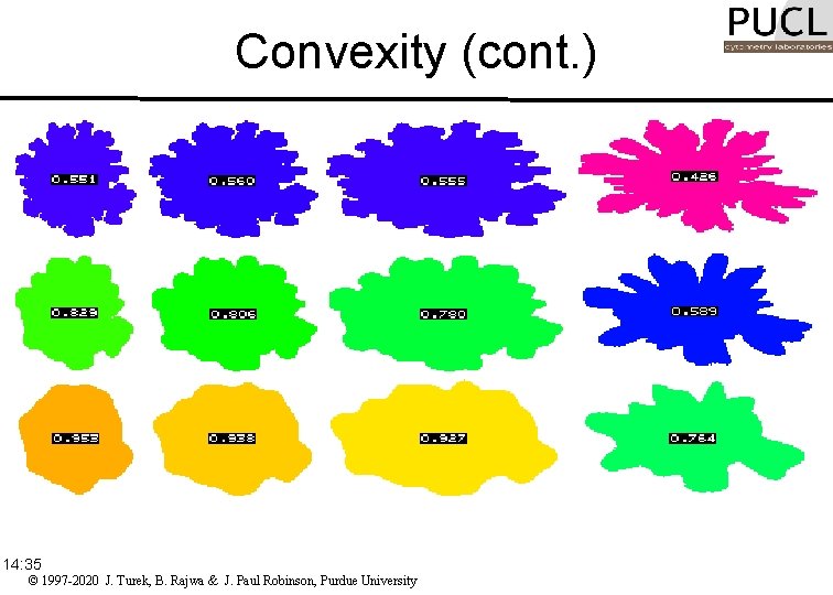
Convexity • Convexity is the relative amount that an object differs from a convex object. A measure of convexity can be obtained by forming the ratio of the perimeter of an object’s convex hull to the perimeter of the object itself: • This will take the value of 1 for a convex object, and will be less than 1 if the object is not convex, such as one having an irregular boundary. 14: 35 © 1997 -2020 J. Turek, B. Rajwa & J. Paul Robinson, Purdue University

Convexity (cont. ) 14: 35 © 1997 -2020 J. Turek, B. Rajwa & J. Paul Robinson, Purdue University

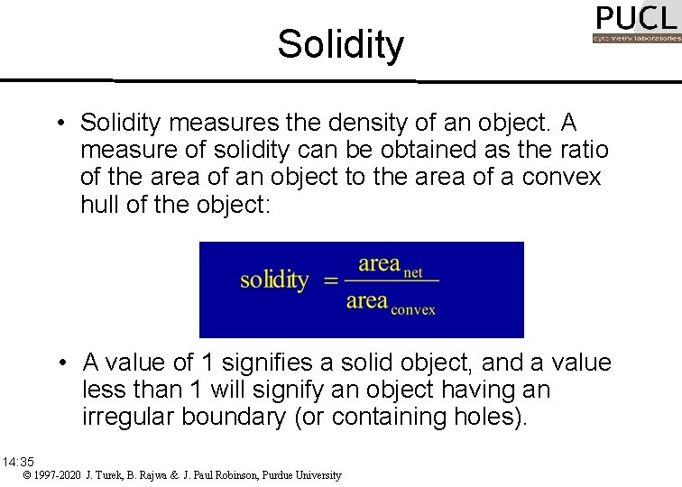
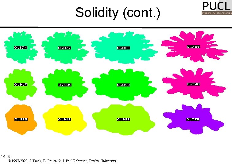
Solidity • Solidity measures the density of an object. A measure of solidity can be obtained as the ratio of the area of an object to the area of a convex hull of the object: • A value of 1 signifies a solid object, and a value less than 1 will signify an object having an irregular boundary (or containing holes). 14: 35 © 1997 -2020 J. Turek, B. Rajwa & J. Paul Robinson, Purdue University

Solidity (cont. ) 14: 35 © 1997 -2020 J. Turek, B. Rajwa & J. Paul Robinson, Purdue University

Moments of shape • The evaluation of moments represents a systematic method of shape analysis. • The most commonly used region attributes are calculated from the three low-order moments. • Knowledge of the low-order moments allows the calculation of the central moments, normalized central moments, and moment invariants. 14: 35 © 1997 -2020 J. Turek, B. Rajwa & J. Paul Robinson, Purdue University

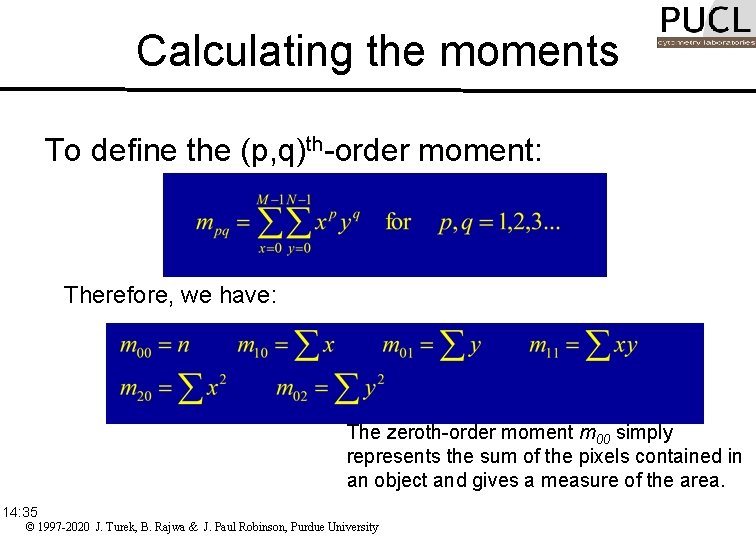
Calculating the moments To define the (p, q)th-order moment: Therefore, we have: The zeroth-order moment m 00 simply represents the sum of the pixels contained in an object and gives a measure of the area. 14: 35 © 1997 -2020 J. Turek, B. Rajwa & J. Paul Robinson, Purdue University

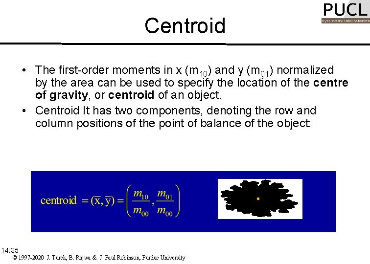
Centroid • The first-order moments in x (m 10) and y (m 01) normalized by the area can be used to specify the location of the centre of gravity, or centroid of an object. • Centroid It has two components, denoting the row and column positions of the point of balance of the object: 14: 35 © 1997 -2020 J. Turek, B. Rajwa & J. Paul Robinson, Purdue University

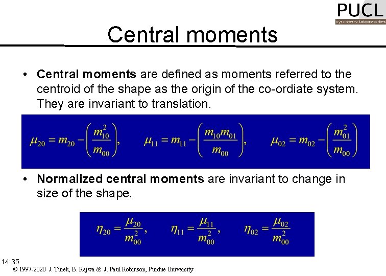
Central moments • Central moments are defined as moments referred to the centroid of the shape as the origin of the co-ordiate system. They are invariant to translation. • Normalized central moments are invariant to change in size of the shape. 14: 35 © 1997 -2020 J. Turek, B. Rajwa & J. Paul Robinson, Purdue University

Moment invariants • Normalisation with respect to orientation results in rotationally invariant moments: • From these, we can calculate the following parameters: 14: 35 © 1997 -2020 J. Turek, B. Rajwa & J. Paul Robinson, Purdue University

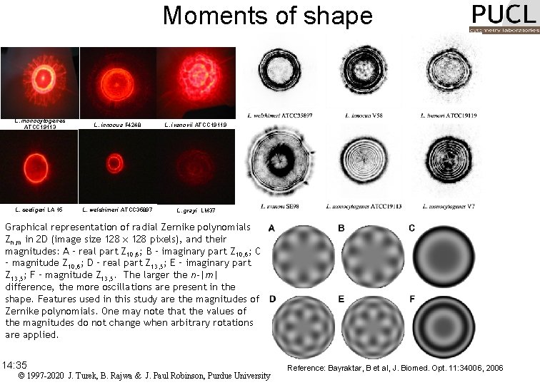
Moments of shape L. monocytogenes ATCC 19113 L. innocua F 4248 L. ivanovii ATCC 19119 L. seeligeri LA 15 L. welshimeri ATCC 35897 L. grayi LM 37 Graphical representation of radial Zernike polynomials Zn, m in 2 D (image size 128 x 128 pixels), and their magnitudes: A – real part Z 10, 6; B – imaginary part Z 10, 6; C – magnitude Z 10, 6; D – real part Z 13, 5; E – imaginary part Z 13, 5; F – magnitude Z 13, 5. The larger the n-|m| difference, the more oscillations are present in the shape. Features used in this study are the magnitudes of Zernike polynomials. One may note that the values of the magnitudes do not change when arbitrary rotations are applied. 14: 35 © 1997 -2020 J. Turek, B. Rajwa & J. Paul Robinson, Purdue University Reference: Bayraktar, B et al, J. Biomed. Opt. 11: 34006, 2006

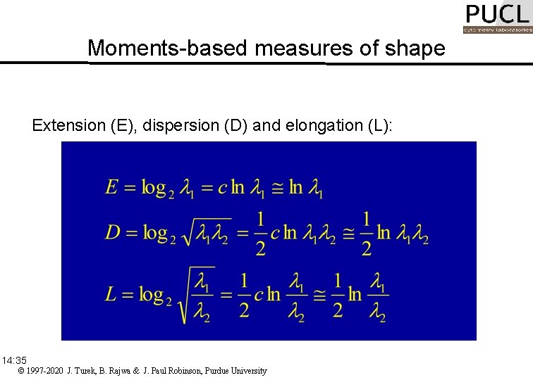
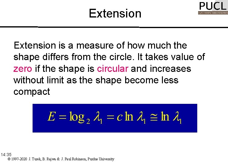
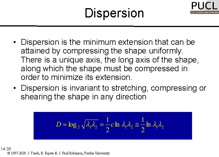
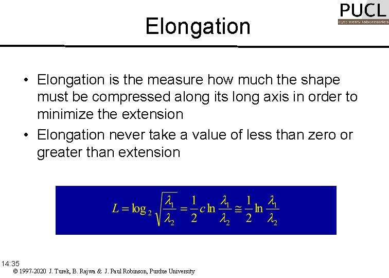
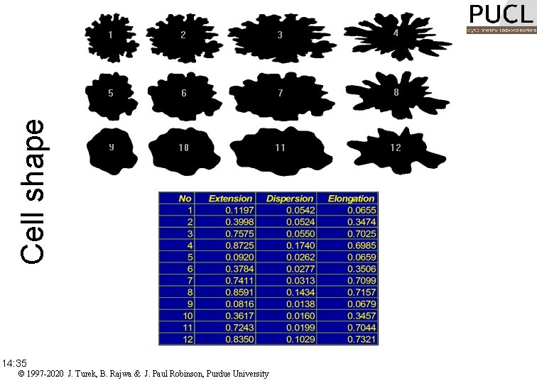
Moments-based measures of shape Extension (E), dispersion (D) and elongation (L): 14: 35 © 1997 -2020 J. Turek, B. Rajwa & J. Paul Robinson, Purdue University

Extension is a measure of how much the shape differs from the circle. It takes value of zero if the shape is circular and increases without limit as the shape become less compact 14: 35 © 1997 -2020 J. Turek, B. Rajwa & J. Paul Robinson, Purdue University

Dispersion • Dispersion is the minimum extension that can be attained by compressing the shape uniformly. There is a unique axis, the long axis of the shape, along which the shape must be compressed in order to minimize its extension. • Dispersion is invariant to stretching, compressing or shearing the shape in any direction 14: 35 © 1997 -2020 J. Turek, B. Rajwa & J. Paul Robinson, Purdue University

Elongation • Elongation is the measure how much the shape must be compressed along its long axis in order to minimize the extension • Elongation never take a value of less than zero or greater than extension 14: 35 © 1997 -2020 J. Turek, B. Rajwa & J. Paul Robinson, Purdue University

Cell shape 14: 35 © 1997 -2020 J. Turek, B. Rajwa & J. Paul Robinson, Purdue University

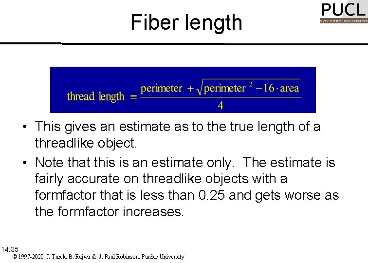
Fiber length • This gives an estimate as to the true length of a threadlike object. • Note that this is an estimate only. The estimate is fairly accurate on threadlike objects with a formfactor that is less than 0. 25 and gets worse as the formfactor increases. 14: 35 © 1997 -2020 J. Turek, B. Rajwa & J. Paul Robinson, Purdue University

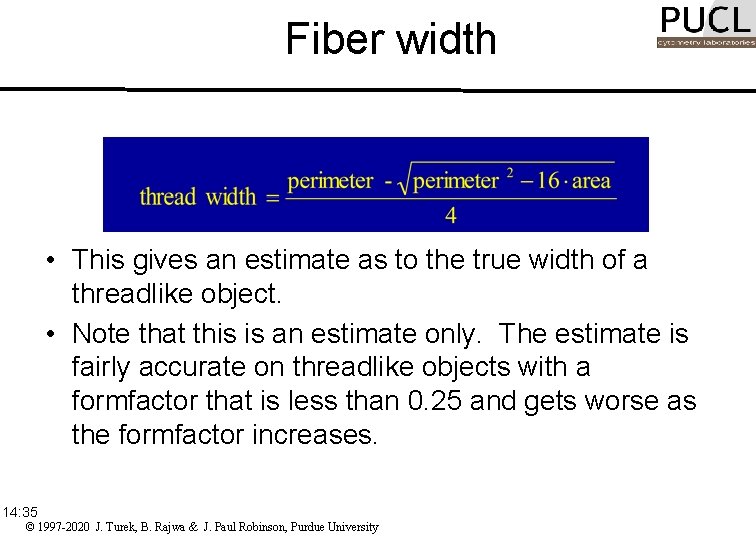
Fiber width • This gives an estimate as to the true width of a threadlike object. • Note that this is an estimate only. The estimate is fairly accurate on threadlike objects with a formfactor that is less than 0. 25 and gets worse as the formfactor increases. 14: 35 © 1997 -2020 J. Turek, B. Rajwa & J. Paul Robinson, Purdue University

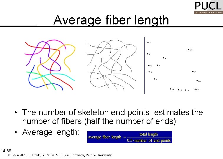
Average fiber length Picture size = 3. 56 in x 3. 56 in Skeletonization Total length = 29. 05 in Number of end-points = 14 • The number of skeleton end-points estimates the number of fibers (half the number of ends) • Average length: Length=4. 15 in 14: 35 © 1997 -2020 J. Turek, B. Rajwa & J. Paul Robinson, Purdue University

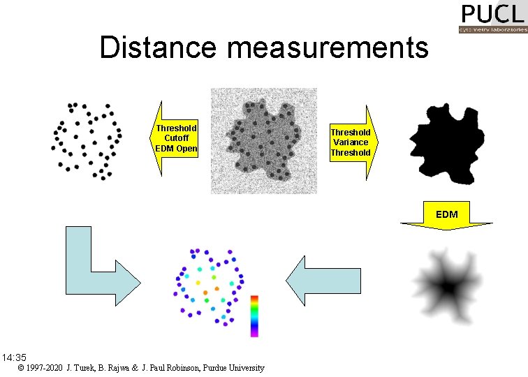
Euclidean distance mapping • Euclidean Distance Map (EDM) converts a binary image to a grey scale image in which pixel value gives the straight-line distance from each originally black pixel within the features to the nearest background (white) pixel. • EDM image can be thresholded to produce erosion, which is both more isotropic and faster than iterative neighbor-based morphological erosion. 14: 35 © 1997 -2020 J. Turek, B. Rajwa & J. Paul Robinson, Purdue University

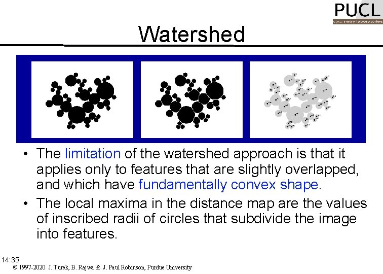
Watershed • The limitation of the watershed approach is that it applies only to features that are slightly overlapped, and which have fundamentally convex shape. • The local maxima in the distance map are the values of inscribed radii of circles that subdivide the image into features. 14: 35 © 1997 -2020 J. Turek, B. Rajwa & J. Paul Robinson, Purdue University

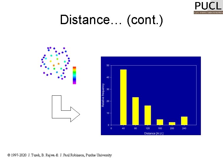
Distance measurements Threshold Cutoff EDM Open Masked result 14: 35 © 1997 -2020 J. Turek, B. Rajwa & J. Paul Robinson, Purdue University Threshold Variance Threshold EDM

Distance… (cont. ) © 1997 -2020 J. Turek, B. Rajwa & J. Paul Robinson, Purdue University

Thresholding • Image thresholding is a segmentation technique which classifies pixels into two categories: – Those to which some property measured from the image falls below a threshold, – and those at which the property equals or exceeds a threshold. • Thesholding creates a binary image (binarisation). 14: 35 © 1997 -2020 J. Turek, B. Rajwa & J. Paul Robinson, Purdue University

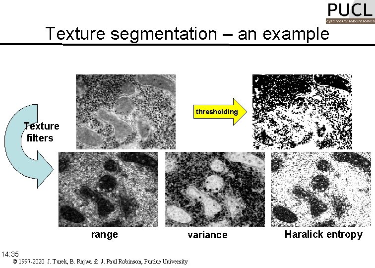
Texture segmentation • Texture is a feature used to partition images into regions of interest and to classify those regions. • Texture provides information about the spatial arrangement of colors or intensities in an image. • Texture is characterized by the spatial distribution of intensity levels in a neighborhood. 14: 35 © 1997 -2020 J. Turek, B. Rajwa & J. Paul Robinson, Purdue University

Texture segmentation – an example thresholding Texture filters range 14: 35 variance © 1997 -2020 J. Turek, B. Rajwa & J. Paul Robinson, Purdue University Haralick entropy

Texture segmentation variance range Original image 14: 35 Texture operator Gaussian Blur © 1997 -2020 J. Turek, B. Rajwa & J. Paul Robinson, Purdue University Haralick entropy Threshold EDM Open, Fill holes

Image math • Image arithmetic on grayscale images (addition, subtraction, division, multiplication, minimum, maximum) • Image Boolean arithmetic (AND, OR, Ex-OR, NOT) 14: 36 © 1997 -2020 J. Turek, B. Rajwa & J. Paul Robinson, Purdue University

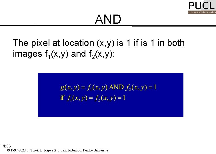
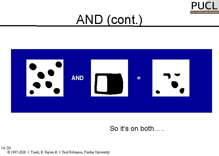
AND The pixel at location (x, y) is 1 if is 1 in both images f 1(x, y) and f 2(x, y): 14: 36 © 1997 -2020 J. Turek, B. Rajwa & J. Paul Robinson, Purdue University

AND (cont. ) AND = So it’s on both…. . 14: 36 © 1997 -2020 J. Turek, B. Rajwa & J. Paul Robinson, Purdue University

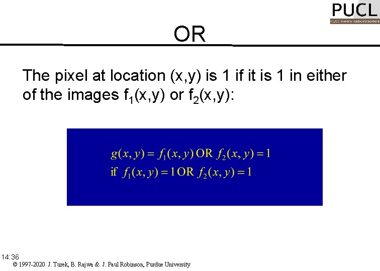
OR The pixel at location (x, y) is 1 if it is 1 in either of the images f 1(x, y) or f 2(x, y): 14: 36 © 1997 -2020 J. Turek, B. Rajwa & J. Paul Robinson, Purdue University

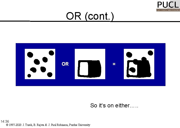
OR (cont. ) OR = So it’s on either…. . 14: 36 © 1997 -2020 J. Turek, B. Rajwa & J. Paul Robinson, Purdue University

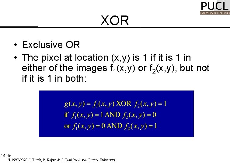
XOR • Exclusive OR • The pixel at location (x, y) is 1 if it is 1 in either of the images f 1(x, y) or f 2(x, y), but not if it is 1 in both: 14: 36 © 1997 -2020 J. Turek, B. Rajwa & J. Paul Robinson, Purdue University

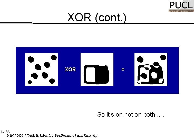
XOR (cont. ) XOR = So it’s on not on both…. . 14: 36 © 1997 -2020 J. Turek, B. Rajwa & J. Paul Robinson, Purdue University

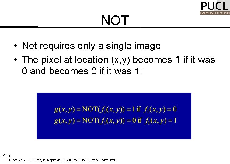
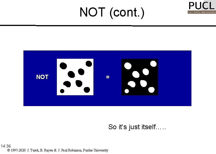
NOT • Not requires only a single image • The pixel at location (x, y) becomes 1 if it was 0 and becomes 0 if it was 1: 14: 36 © 1997 -2020 J. Turek, B. Rajwa & J. Paul Robinson, Purdue University

NOT (cont. ) NOT = So it’s just itself…. . 14: 36 © 1997 -2020 J. Turek, B. Rajwa & J. Paul Robinson, Purdue University

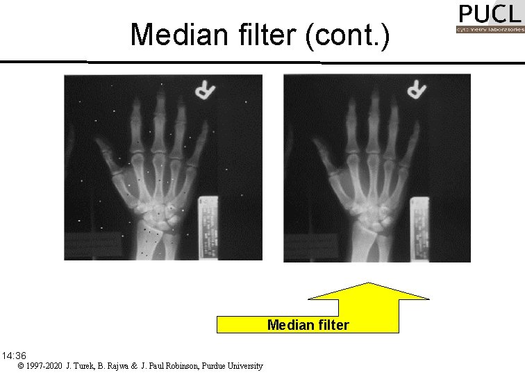
Non-linear filters • Non-linear filters are known collectively as order statistic filters or rank filters • How does it work? Let’s combine a list of intensity values in the neighborhood of a given pixel, sort the list into ascending order, then select a value from a particular position in the list to use as the new value for the pixel. 14: 36 © 1997 -2020 J. Turek, B. Rajwa & J. Paul Robinson, Purdue University

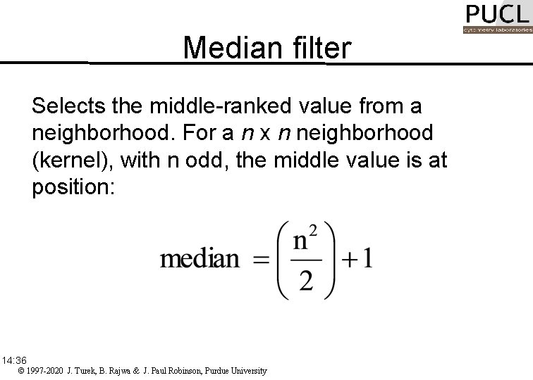
Median filter Selects the middle-ranked value from a neighborhood. For a n x n neighborhood (kernel), with n odd, the middle value is at position: 14: 36 © 1997 -2020 J. Turek, B. Rajwa & J. Paul Robinson, Purdue University

Median filter (cont. ) + Median filter 14: 36 © 1997 -2020 J. Turek, B. Rajwa & J. Paul Robinson, Purdue University

Periodic Noise Periodic noise in an image may be removed by editing a 2 -dimensional Fourier transform (FFT). A forward FFT of the image below, will allow you to view the periodic noise (center panel) in an image. This noise, as indicated by the white box, may be edited from the image and then an inverse Fourier transform performed to restore the image without the noise (right panel next slide). 14: 36 © 1997 -2020 J. Turek, B. Rajwa & J. Paul Robinson, Purdue University

Pseudocolor image based upon gray scale or luminance Human vision more sensitive to color. Pseudocoloring makes it is possible to see slight variations in gray scales 14: 36 © 1997 -2020 J. Turek, B. Rajwa & J. Paul Robinson, Purdue University

See previous lecture • • 14: 36 Nyquist Theory To sample or graph a SINE wave you must have at least two points or coordinates in order to guess what the frequency is. . For example you need the ORIGIN (y=0 normally) and either a MAXIMUM or a MINIMUM value to guess the frequency. Because of this simple fact, to record a frequency you must have at least double that number as the sampling rate. . EG. To record a sine wave of 50 Hz you need a MINIMUM of 100 samples per second to record the sine wave. This basic fact which governs the minimum sampling rate is called the Nyquist theory. The Nyquist frequency is the highest frequency that you can record with a given sample rate. In the case of a recording with 44, 100 samples per second (the sampling rate of CDs) the Nyquist frequency is 22050 Hz. I could go in to drawing pictures to prove this but I wont because you have seen the quality of my drawings above. LOL. The Nyquist theory is not something that you will hear much about but is good to know what it is and how it effects things in real life situations. © 1997 -2020 J. Turek, B. Rajwa & J. Paul Robinson, Purdue University

Manipulating Images for publication • …we teach you how to manipulate images • …. But we also know how to determine if you did cheat!!. . • To be expanded in a separate lecture! 14: 36 © 1997 -2020 J. Turek, B. Rajwa & J. Paul Robinson, Purdue University

Conclusion & Summary • Image Collection – resolution and physical determinants of collection instrument – collect only what you actually need • Image Processing – thresholding, noise reduction, filtering, histogram manipulation, etc • Image Analysis – feature identification, segmentation, value of data, representation of image, extract arithmetic information • Must not exceed an acceptable scientific standard in modification of images • If you cheat and publish, its there for everyone to see…someone smarter than you may dig into your data and expose you!! © 1997 -2020 J. Turek , B. Rajwa & J. Paul Robinson, Purdue University