Principles for teaching and using Bayes factors Zoltn

Principles for teaching and using Bayes factors Zoltán Dienes

I Bayes factors in context: The problem to be solved II Anatomy of a Bayes factor III Criticisms of Bayes factors

I Bayes factors in context: The problem to be solved

Inferential statistics: 1. Estimation: How much? 2. Hypothesis testing: Does it exist?

Questions asking for estimation: 1. What proportion of Americans would vote for Trump now? 2. How strong is the relation between daily exercise and heart rate?

Questions asking for estimation: 1. What proportion of Americans would vote for Trump now? 2. How strong is the relation between daily exercise and heart rate? Cf: Is there a relation?
: We want (given doubt about something’s existence) evidence for")
A common view (and mine): We want (given doubt about something’s existence) evidence for whether it exists AND (given that something credibly exists) to estimate how big it is Counter view: Only estimate! Andrew Gelman John Kruschke Geoff Cumming

Was there any conscious perception of the stimulus? Do people perform above baseline? Was the ERP higher for grammatical than non-grammatical stimuli? Does rewarding eating greens make greens less desirable?

Was there any conscious perception of the stimulus? Do people perform above baseline? Was the ERP higher for grammatical than non-grammatical stimuli? Does rewarding eating greens make greens less desirable? Could we settle for an estimate rather than a hypothesis test?

Do people perform above chance?

Do people perform above chance? Estimation with frequentist statistics: Confidence interval: Accept as possible population values those within the interval; reject those without Estimation with Bayes: Credibility interval: Probability that population value lies between two values
 95% Confidence interval is: 45% -")
Do people perform above chance? (chance is 50%) 95% Confidence interval is: 45% - 55% Can we conclude that people performed at chance?

If the point null can never be affirmed by estimation … Make a null region: Null region 50% Minimal interesting effect size
: Null region Minimal interesting value")
The four principles of inference by intervals (Dienes, 2014): Null region Minimal interesting value 0 Difference between means -> Lakens – equivalence testing accept the null region hypothesis reject a directional theory Data are insensitive: suspend judgment

Problems: 1. Need to specify a minimally interesting effect size in a non-arbitrary way Consider: For claiming a stimulus is subliminal, what level of discrimination accuracy is too small to be interesting?

Problems: 1. Need to specify a minimally interesting effect size in a non-arbitrary way Consider: For claiming a stimulus is subliminal, what level of discrimination accuracy is too small to be interesting? NB Armstrong & Dienes 2014 found 52% for discriminating degraded stimuli and concluded performance was above an objective threshold

Problems: 1. Need to specify a minimally interesting effect size in a non-arbitrary way Consider: For claiming a stimulus is subliminal, what level of discrimination is too small to be interesting? 2. Plausible answers to 1. imply null regions requiring a truck load of subjects to allow squeezing an interval in. Consider: Say 51% is small enough (is there an objective reason for this? ) So null region is 49% - 51%

Sample SE = 1. 78 with 27 subjects If sample mean = 50% would need SE = 0. 5% (limit of CI = sample mean + 2×SE ) Lower Limit 2×SE Sample Mean 2×SE Upper limit i. e. SE needs to be about quarter of what was found So would need 42 x 27 = about 400 subjects.

Problems with inference by intervals: 1. Need to specify a minimally interesting effect size in a non-arbitrary way 2. Plausible answers to 1. imply null regions requiring a truck load of subjects to allow squeezing an interval in. MORAL: The attempt to smuggle in hypothesis testing to estimation does not provide a general solution

So use hypothesis testing! Significance testing?

Evidence for H 0 No evidence to speak of Evidence for H 1

P-values make a two distinction: Evidence for H 0 No evidence to speak of NO MATTER WHAT THE P-VALUE, NO DISTINCTION MADE WITHIN THIS BOX Evidence for H 1

What to take from those pushing estimation: If there is no doubt that something exists, just estimate E. g. Correlation between two measure of same thing Performance on a task that obviously people will learn

What to take from those pushing estimation: If there is no doubt that something exists, just estimate E. g. Correlation between two measure of same thing Performance on a task that obviously people will learn If you do estimate SAY: “Performance is probably between 45% and 65%” DO NOT SAY: “And therefore people are at chance”

Main message: Estimation does not allow us to get evidence for no effect. Significance testing does not either. We need something else …

II Anatomy of a Bayes factor
 P(H 0 | D) =")
From the axioms of probability: P(H 1 | D) P(H 0 | D) = Posterior confidence = P(D | H 1) P(D | H 0) × P(H 1) P(H 0) Bayes factor × prior confidence in H 1 rather than H 0 Defining strength of evidence by the amount one’s belief ought to change, Bayes factor is a measure of strength of evidence

If B = about 1, experiment was not sensitive. If B > 1 then the data supported your theory over the null If B < 1, then the data supported the null over your theory Jeffreys, 1939: Bayes factors more than 3 are worth taking note of Taking note of = Worth exploring further? B > 3 noticeable support for H 1 over null B < 1/3 noticeable support for null over H 1
 Bayes factors make three way distinction: 0")
(given an agreed strength of evidence k) Bayes factors make three way distinction: 0 … 1/k Evidence for H 0 1/k … k No evidence to speak of k… Evidence for H 1
 means: Can get evidence for H 0")
The symmetry of B (and not p) means: Can get evidence for H 0 just as much for H 1 - help against publication bias - allow claimed evidence against H 1 only when there is Can run until evidence is strong enough (Optional stopping no longer a QRP) Less pressure to B-hack – and when it occurs can go in either direction.
 P(H 0 | D) =")
From the axioms of probability: P(H 1 | D) P(H 0 | D) = Posterior confidence = P(D | H 1) P(D | H 0) × P(H 1) P(H 0) Bayes factor × prior confidence in H 1 rather than H 0 Defining strength of evidence by the amount one’s belief ought to change, Bayes factor is a measure of strength of evidence

A model of H 0

A model of H 0 A model of the data

A model of H 0 A model of the data A model of H 1

Is there an animal in the room?
 animal in the room? Different models of H 1 Good")
Is there an (unobstructed) animal in the room? Different models of H 1 Good evidence there is not! Evidence not clear ….

Is there an animal in the room? Need to increase number of subjects … NB : standard error is in model of data Now can pick up smaller effects

Evidence for something not being there depends on model of what could be there Whether Bayesian or otherwise, saying there is no signal depends on how big a signal we expect relative to the noise. We must have a model of H 1 to get evidence for a point null.

How do we model the predictions of H 1? How to derive predictions from a theory? Theory Predictions

How do we model the predictions of H 1? How to derive predictions from a theory? Theory assumptions Predictions

How do we model the predictions of H 1? How to derive predictions from a theory? Theory assumptions Predictions Want assumptions that are a) informed; and b) simple

How do we model the predictions of H 1? How to derive predictions from a theory? Theory assumptions Model of predictions Plausibility Magnitude of effect Want assumptions that are a) informed; and b) simple

Example Initial study: Meditating on breathing for 20 minutes a day over two weeks increases self-rated mindfulness by 0. 6 of a point on a 1 -5 scale. Follow up Study: Meditating on walking instead of breathing for 20 minutes a day; other details same. What size effect could be expected?
: Published studies tend to have larger")
A point to consider: Reproducibility project (osf, 2015): Published studies tend to have larger effect sizes than unbiased direct replications; Original effect size Replication effect size Psychology Behavioural economics

1. Assume a measured effect size is roughly right scale of effect 2. Assume smaller effects more likely than bigger ones => Rule of thumb: If initial raw effect is E, then assume half-normal with SD = E Plausibility Possible population mean differences

Example Initial study: Focusing on breathing for 20 minutes a day over two weeks increases self-rated mindfulness by 0. 6 of a point on a 1 -5 scale (from 3 to 3. 6) t(30) = 2. 10, p = 0. 044, Cohen’s d = 0. 74 Follow up Study: Walking mediation How should we model H 1? Roughly 0. 6 unit effect expected.
 New study: 0. 36 rating units, SE = 0. 18,")
half-normal H(0, 0. 6) New study: 0. 36 rating units, SE = 0. 18, t(88) = 2. 00, p =. 049 BH(0, 0. 6) = 3. 50

Initial study: 0. 2 units on a 1 -5 scale (from 3 to 3. 2), p = 0. 044 Initial study: 1. 5 units on a 1 -5 scale (from 2 to 3. 5), p = 0. 044 New study: 0. 1 units, SE = 0. 3, t(88) = 0. 33, p = 0. 74 BH(0, 0. 2) = BH(0, 1. 5) =

Initial study: 0. 2 units on a 1 -5 scale (from 3 to 3. 2), p = 0. 044 Initial study: 1. 5 units on a 1 -5 scale (from 2 to 3. 5), p = 0. 044 New study: 0. 1 units, SE = 0. 3, t(88) = 0. 33, p = 0. 74 BH(0, 0. 2) = 0. 97 BH(0, 1. 5) = 0. 26

V Criticisms of Bayes factors: 1. Different models of H 1 give different answers 2. A default Bayes factor is not relevant to your theory 3. The point H 0 is never true 4. Bayes factors don’t control error rates

1. Different models of H 1 give different answers If H 1 is modelled according to someone’s personal belief, why should anyone else take any notice of the Bayes factor? My personal belief may give different answers. (Argument against subjective Bayes. )

1. Different models of H 1 give different answers If H 1 is modelled according to someone’s personal belief, why should anyone else take any notice of the Bayes factor? My personal belief may give different answers. (Argument against subjective Bayes. ) Answer: Choices (e. g. parameter values) should be based on publicly available reasons for their relevance to the scientific context. (WHY SD = 0. 6 rating units? Because THIS study got that effect. )

1. Different models of H 1 give different answers If H 1 is modelled according to someone’s personal belief, why should anyone else take any notice of the Bayes factor? My personal belief may give different answers. (Argument against subjective Bayes. ) Answer: Choices (e. g. parameter values) should be based on publicly available reasons for their relevance to the scientific context. (WHY SD = 0. 6 rating units? Because THIS study got that effect. ) Then one makes a judgment that the representation is adequate for the scientific context (and aims to convince one’s peers to do likewise)

Initial study: Focusing on breathing for 20 minutes a day over two weeks increases self-rated mindfulness by 0. 6 of a point on a 1 -5 scale (from 3 to 3. 6) Follow up Study: Walking instead of breathing meditation Result: Meditation increases mindfulness by 0. 36 units, SE = 0. 14 BH(0, 0. 6) = 10. 39 BH(0, 0. 068) = 2. 94 BH(0, 2. 6) = 2. 89

Initial study: Focusing on breathing for 20 minutes a day over two weeks increases self-rated mindfulness by 0. 6 of a point on a 1 -5 scale (from 3 to 3. 6) Follow up Study: Walking instead of breathing meditation Result: Meditation increases mindfulness by 0. 36 units, SE = 0. 14 BH(0, 0. 6) = 10. 39 BH(0, 0. 068) = 2. 94 BH(0, 2. 6) = 2. 89 Have to scale BH below 0. 07 or above 2. 5 units to get B < 3 As these limits exceed judgment of what is reasonable, conclusion is robust. Report robustness region: RR[0. 07, 2. 5] (thanks to Balazs Aczel)

2. A default Bayes factor is not relevant to your theory. (Argument against objective Bayes) Right. Make sure your model of H 1 is relevant to your theory. (Always specify what your model of H 1 is and give an objective reason why you set any parameter. )

3. The point null is never true; therefore only thing to do is estimation From Baguley (2012): Wiseman and Greening (2002) Online experiment with 27, 856 participants testing existence of ESP with a chance baseline of 50%. 95% CI [49. 6%, . 50. 2%] So true null may be an interval [-. 3%, +. 3%] around 50%

Result just gives support for H 1: 55% correct SE = 2. 5% BH(0, 5) = 4. 27 against point null BH(0, 5) = 4. 19 against interval null [-0. 5%, +0. 5%] around 50% The point null will often be a perfectly adequate approximation in well-controlled experimental research

4. A Bayes factor does not control error rates. A Bayes factor fixes strength of evidence; What you do with evidence (over many cases) determines error rates Fixing one does not fix the other. Who ate the cakes? Evidence not error rates is how much you should change your confidence in H 1 versus H 0. See Dienes 2016 JMP

Evidence constrains error rates without fixing them Just as an object constrains but does not fix shadows. The more the evidence the less the errors in total. (Maybe we need a higher B threshold than we have been used to. )

There are no arguments against Bayes factors Only against their misuse or misunderstanding

To obtain evidence for a point null hypothesis one must use Bayes factors One moral: Never say there was “no effect of. . “, never discuss why there was no effect, when all you have reported is nonsignificance

Teaching undergrads: 1. Use estimation alone if there being some effect is not in doubt. 2. To answer an existential question (effect in doubt but an interesting theory postulates the effect), use Bayes factors: Think carefully about scientific context and range of raw effect sizes that are reasonable. 3. “Significance” is useful as indicating there is some model of H 1 for which there is evidence over H 0. Worth knowing, but no substitute for knowing one’s science.

http: //www. lifesci. sussex. ac. uk/home/Zoltan_Dienes/ Model H 1 with uniform or normal distributions; raw or standardized effect sizes; can centre on zero or elsewhere

https: //medstats. github. io/bayesfactor. html Model H 1 with uniform, normal, t, or Cauchy distributions; raw or standardised effect sizes; can centre on zero or elsewhere

http: //pcl. missouri. edu/bayesfactor Model H 1 with Cauchy; standardised effect size; centred on zero


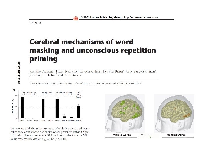
ERP components and f. MRI response in left fusiform and extrastriate cortex reduced to 5 – 20% for masked words compared to consciously seen words. Þ So we might expect discrimination to be 10% of that possible with conscious words

Priming = 5%, p <. 05; classification = 51%, p >. 05. Conscious classification = 100% 5% Unconscious priming = 10% of P Conscious priming, P So if conscious classification = 70% and conscious priming is twice unconscious priming…

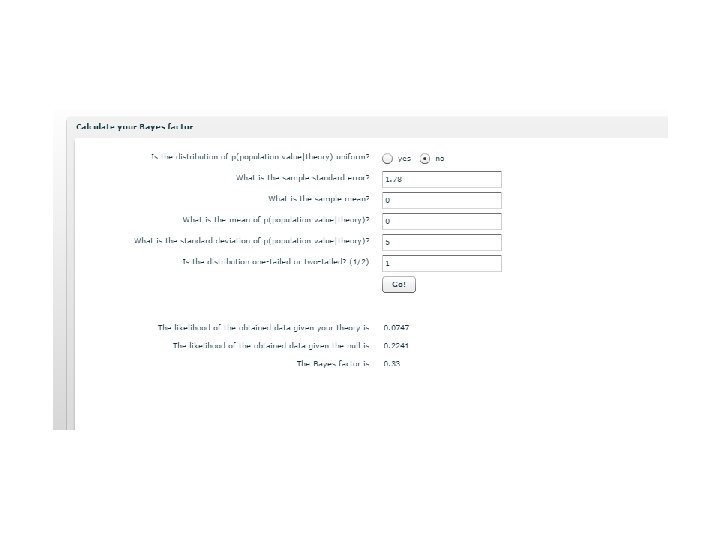
ERP components and f. MRI response in left fusiform and extrastriate cortex reduced to 5 – 20% for masked words compared to consciously seen words. Þ So we might expect discrimination to be 10% of that possible with conscious words Actual discrimination was 52. 9% i. e. 2. 9% above baseline, t = 1. 63 SE = (mean diff)/t = 2. 9%/1. 63 = 1. 78% Sample mean = 2. 9, sample SE = 1. 78

B = 2. 04 Objective threshold not established
- Slides: 74