Principal Components An Introduction exploratory factoring meaning application

Principal Components An Introduction • exploratory factoring • meaning & application of “principal components” • Basic steps in a PC analysis • PC extraction process • PC rotation & interpretation • # PCs determination • “Kinds” of factors and variables • selecting and “accepting” data sets

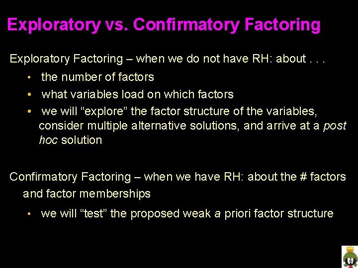
Exploratory vs. Confirmatory Factoring Exploratory Factoring – when we do not have RH: about. . . the number of factors • what variables load on which factors • we will “explore” the factor structure of the variables, consider multiple alternative solutions, and arrive at a post hoc solution • Confirmatory Factoring – when we have RH: about the # factors and factor memberships • we will “test” the proposed weak a priori factor structure

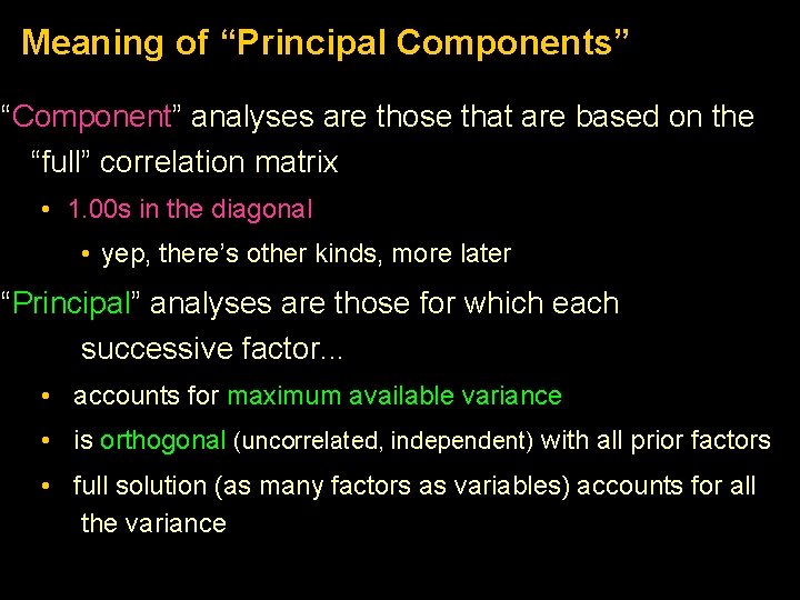
Meaning of “Principal Components” “Component” analyses are those that are based on the “full” correlation matrix • 1. 00 s in the diagonal • yep, there’s other kinds, more later “Principal” analyses are those for which each successive factor. . . • accounts for maximum available variance • is orthogonal (uncorrelated, independent) with all prior factors • full solution (as many factors as variables) accounts for all the variance

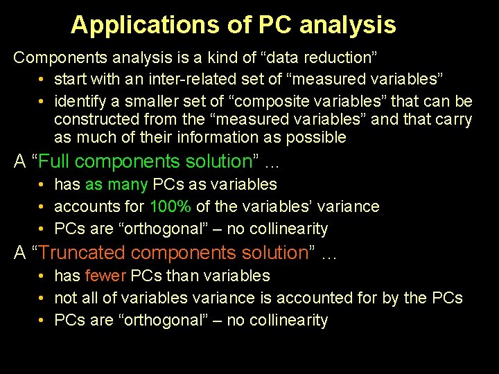
Applications of PC analysis Components analysis is a kind of “data reduction” • start with an inter-related set of “measured variables” • identify a smaller set of “composite variables” that can be constructed from the “measured variables” and that carry as much of their information as possible A “Full components solution”. . . • has as many PCs as variables • accounts for 100% of the variables’ variance • PCs are “orthogonal” – no collinearity A “Truncated components solution” … • has fewer PCs than variables • not all of variables variance is accounted for by the PCs • PCs are “orthogonal” – no collinearity

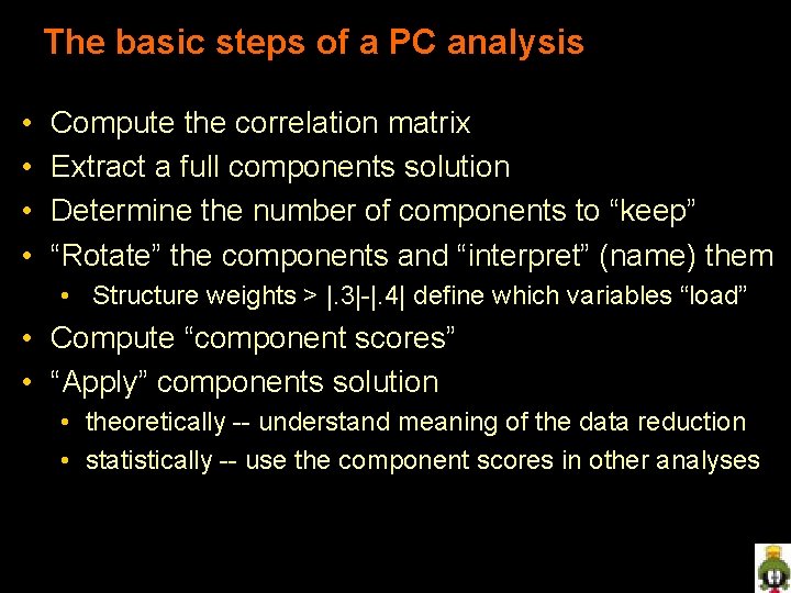
The basic steps of a PC analysis • • Compute the correlation matrix Extract a full components solution Determine the number of components to “keep” “Rotate” the components and “interpret” (name) them • Structure weights > |. 3|-|. 4| define which variables “load” • Compute “component scores” • “Apply” components solution • theoretically -- understand meaning of the data reduction • statistically -- use the component scores in other analyses

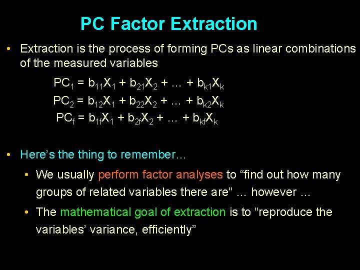
PC Factor Extraction • Extraction is the process of forming PCs as linear combinations of the measured variables PC 1 = b 11 X 1 + b 21 X 2 + … + bk 1 Xk PC 2 = b 12 X 1 + b 22 X 2 + … + bk 2 Xk PCf = b 1 f. X 1 + b 2 f. X 2 + … + bkf. Xk • Here’s the thing to remember… • We usually perform factor analyses to “find out how many groups of related variables there are” … however … • The mathematical goal of extraction is to “reproduce the variables’ variance, efficiently”

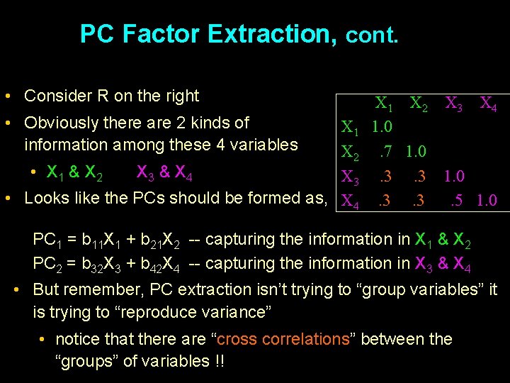
PC Factor Extraction, cont. • Consider R on the right • Obviously there are 2 kinds of information among these 4 variables X 1 X 2 • X 1 & X 2 X 3 & X 4 X 3 • Looks like the PCs should be formed as, X 4 X 1 X 2 X 3 X 4 1. 0. 7 1. 0. 3. 3. 5 1. 0 PC 1 = b 11 X 1 + b 21 X 2 -- capturing the information in X 1 & X 2 PC 2 = b 32 X 3 + b 42 X 4 -- capturing the information in X 3 & X 4 • But remember, PC extraction isn’t trying to “group variables” it is trying to “reproduce variance” • notice that there are “cross correlations” between the “groups” of variables !!

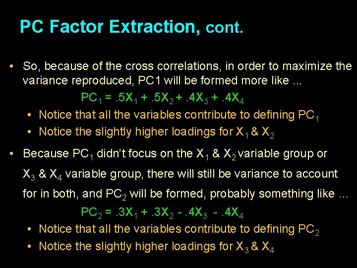
PC Factor Extraction, cont. • So, because of the cross correlations, in order to maximize the variance reproduced, PC 1 will be formed more like. . . PC 1 =. 5 X 1 +. 5 X 2 +. 4 X 3 +. 4 X 4 • Notice that all the variables contribute to defining PC 1 • Notice the slightly higher loadings for X 1 & X 2 • Because PC 1 didn’t focus on the X 1 & X 2 variable group or X 3 & X 4 variable group, there will still be variance to account for in both, and PC 2 will be formed, probably something like … PC 2 =. 3 X 1 +. 3 X 2 -. 4 X 3 -. 4 X 4 • Notice that all the variables contribute to defining PC 2 • Notice the slightly higher loadings for X 3 & X 4

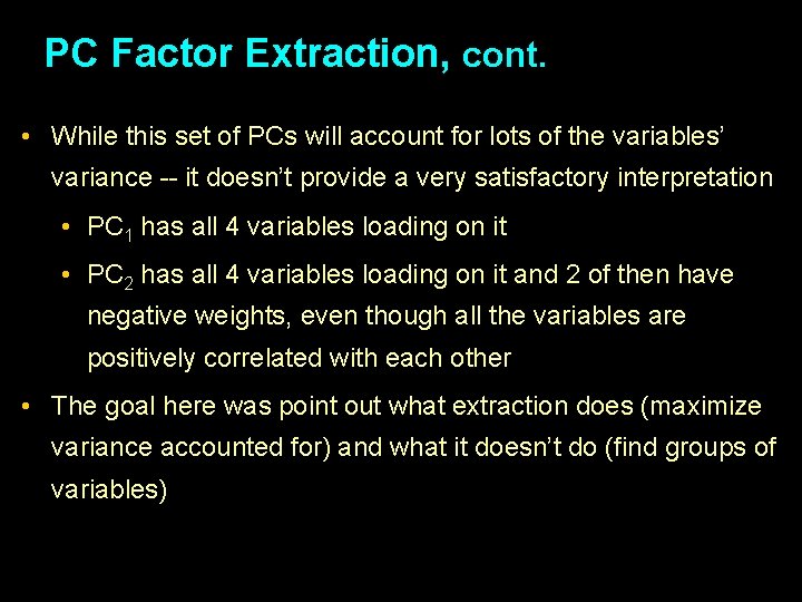
PC Factor Extraction, cont. • While this set of PCs will account for lots of the variables’ variance -- it doesn’t provide a very satisfactory interpretation • PC 1 has all 4 variables loading on it • PC 2 has all 4 variables loading on it and 2 of then have negative weights, even though all the variables are positively correlated with each other • The goal here was point out what extraction does (maximize variance accounted for) and what it doesn’t do (find groups of variables)

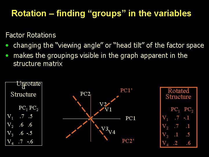
Rotation – finding “groups” in the variables Factor Rotations • changing the “viewing angle” or “head tilt” of the factor space • makes the groupings visible in the graph apparent in the structure matrix Unrotate d Structure V 1 V 2 V 3 V 4 PC 1 PC 2. 7. 5. 6. 6. 6 -. 5. 7 -. 6 PC 1’ PC 2 Rotated Structure V 2 V 1 PC 1 V 3 V 4 PC 2’ V 1 V 2 V 3 V 4 PC 1 PC 2. 7 -. 1. 7. 1. 1. 5. 2. 6

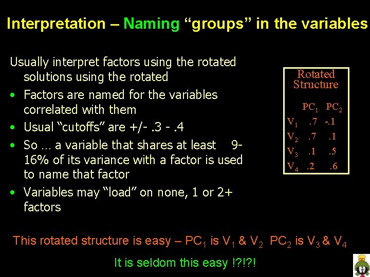
Interpretation – Naming “groups” in the variables Usually interpret factors using the rotated solutions using the rotated • Factors are named for the variables correlated with them • Usual “cutoffs” are +/-. 3 -. 4 • So … a variable that shares at least 916% of its variance with a factor is used to name that factor • Variables may “load” on none, 1 or 2+ factors Rotated Structure V 1 V 2 V 3 V 4 PC 1 PC 2. 7 -. 1. 7. 1. 1. 5. 2. 6 This rotated structure is easy – PC 1 is V 1 & V 2 PC 2 is V 3 & V 4 It is seldom this easy !? !? !

Determining the Number of PCs Determining the number of PCs is arguably the most important decision in the analysis … • rotation, interpretation and use of the PCs are all influenced by the how may PCs are “kept” for those processes • there are many different procedures available – none are guaranteed to work !! • probably the best approach to determining the # of PCS… • remember that this is an exploratory factoring -- that means you don’t have decent RH: about the number of factors • So … Explore … • consider different “reasonable” # PCs and “try them out” • rotate, interpret &/or tryout resulting factor scores from each and then decide To get started we’ll use the SPSS “standard” of λ > 1. 00

Mathematical Procedures • The most commonly applied decision rule (and the default in most stats packages -- chicken & egg ? ) is the > 1. 00 rule … here’s the logic • Any PC with > 1. 00 accounts for more variance than the average variable in that R • That PC “has parsimony” -- the more complex composite has more information than the average variable • Any PC with < 1. 00 accounts for less variance than the average variable in that R • That PC “doesn’t have parsimony”

Statistical Procedures • PC analyses are extracted from a correlation matrix • PCs should only be extracted if there is “systematic covariation” in the correlation matrix • This is know as the “sphericity question” • Note: the test asks if there the next PC should be extracted • There are two different sphericity tests • Whethere is any systematic covariation in the original R • Whethere is any systematic covariation left in the partial R, after a given number of factors has been extracted • Both tests are called “Bartlett’s Sphericity Test”

Statistical Procedures, cont. • Applying Bartlett’s Sphericity Tests • Retaining H 0: means “don’t extract another factor” • Rejecting H 0: means “extract the next factor” • Significance tests provide a p-value, and so a known probability that the next factor is “ 1 too many” (a type I error) • Like all significance tests, these are influenced by “N” • larger N = more power = more likely to reject H 0: = more likely to “keep the next factor” (& make a Type I error) • Quandary? !? • Samples large enough to have a stable R are likely to have “excessive power” and lead to “over factoring” • Be sure to consider % variance, replication & interpretability

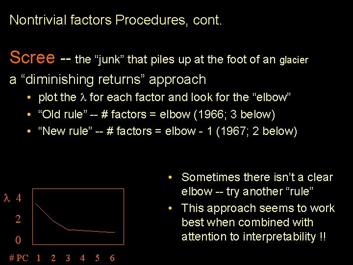
Nontrivial factors Procedures, cont. Scree -- the “junk” that piles up at the foot of an glacier a “diminishing returns” approach • plot the for each factor and look for the “elbow” • “Old rule” -- # factors = elbow (1966; 3 below) • “New rule” -- # factors = elbow - 1 (1967; 2 below) • Sometimes there isn’t a clear elbow -- try another “rule” • This approach seems to work best when combined with attention to interpretability !! 4 2 0 # PC 1 2 3 4 5 6

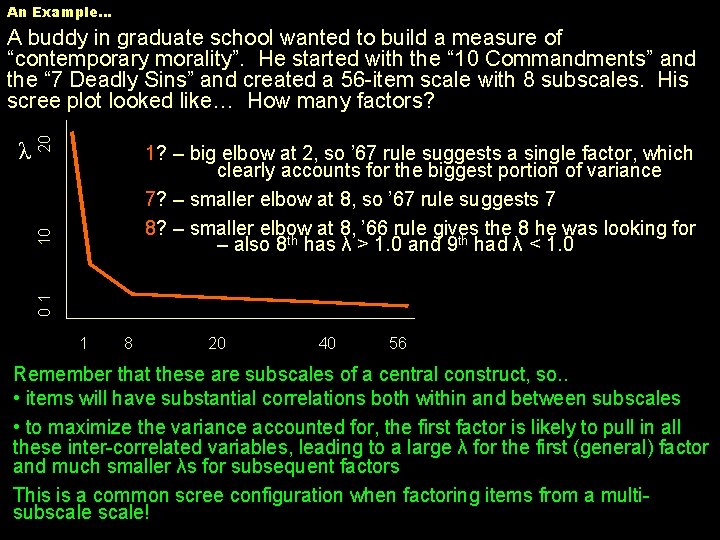
An Example… 1? – big elbow at 2, so ’ 67 rule suggests a single factor, which clearly accounts for the biggest portion of variance 7? – smaller elbow at 8, so ’ 67 rule suggests 7 8? – smaller elbow at 8, ’ 66 rule gives the 8 he was looking for – also 8 th has λ > 1. 0 and 9 th had λ < 1. 0 01 10 λ 20 A buddy in graduate school wanted to build a measure of “contemporary morality”. He started with the “ 10 Commandments” and the “ 7 Deadly Sins” and created a 56 -item scale with 8 subscales. His scree plot looked like… How many factors? 1 8 20 40 56 Remember that these are subscales of a central construct, so. . • items will have substantial correlations both within and between subscales • to maximize the variance accounted for, the first factor is likely to pull in all these inter-correlated variables, leading to a large λ for the first (general) factor and much smaller λs for subsequent factors This is a common scree configuration when factoring items from a multisubscale!

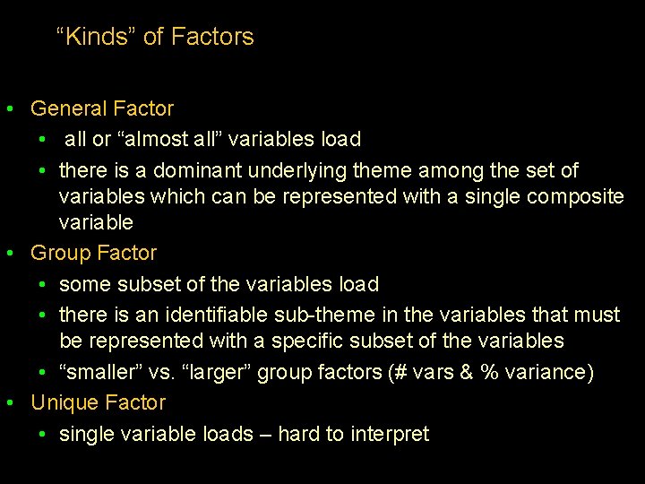
“Kinds” of Factors • General Factor • all or “almost all” variables load • there is a dominant underlying theme among the set of variables which can be represented with a single composite variable • Group Factor • some subset of the variables load • there is an identifiable sub-theme in the variables that must be represented with a specific subset of the variables • “smaller” vs. “larger” group factors (# vars & % variance) • Unique Factor • single variable loads – hard to interpret

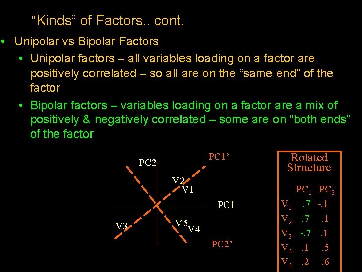
“Kinds” of Factors. . cont. • Unipolar vs Bipolar Factors • Unipolar factors – all variables loading on a factor are positively correlated – so all are on the “same end” of the factor • Bipolar factors – variables loading on a factor are a mix of positively & negatively correlated – some are on “both ends” of the factor PC 1’ PC 2 Rotated Structure V 2 V 1 PC 1 V 3 V 5 V 4 PC 2’ V 1 V 2 V 3 V 4 PC 1. 7. 7 -. 7. 1. 2 PC 2 -. 1. 1. 1. 5. 6

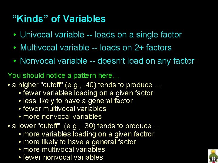
“Kinds” of Variables • Univocal variable -- loads on a single factor • Multivocal variable -- loads on 2+ factors • Nonvocal variable -- doesn’t load on any factor You should notice a pattern here… • a higher “cutoff” (e. g. , . 40) tends to produce … • fewer variables loading on a given factor • less likely to have a general factor • fewer multivocal variables • more nonvocal variables • a lower “cutoff” (e. g. , . 30) tends to produce … • more variables loading on a given factror • more likely to have a general factor • more multivocal variables • fewer nonvocal variables

Selecting Variables for a Factor Analysis • The variables in the analysis determine the analysis results • this has been true in every model we’ve looked at (remember how the inclusion of covariate and/or interaction terms has radically changed some results we’ve seen) • this is very true of factor analysis, because the goal is to find “sets of variables” • Variable sets for factoring come in two “kinds” • when the researcher has “hand-selected” each variable • when the researcher selects a “closed set” of variables (e. g. , the sub-scales of a standard inventory, the items of an interview, or the elements of data in a “medical chart”)

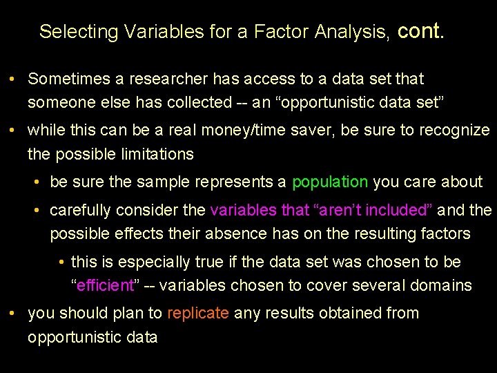
Selecting Variables for a Factor Analysis, cont. • Sometimes a researcher has access to a data set that someone else has collected -- an “opportunistic data set” • while this can be a real money/time saver, be sure to recognize the possible limitations • be sure the sample represents a population you care about • carefully consider the variables that “aren’t included” and the possible effects their absence has on the resulting factors • this is especially true if the data set was chosen to be “efficient” -- variables chosen to cover several domains • you should plan to replicate any results obtained from opportunistic data

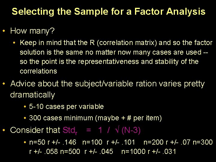
Selecting the Sample for a Factor Analysis • How many? • Keep in mind that the R (correlation matrix) and so the factor solution is the same no matter now many cases are used -so the point is the representativeness and stability of the correlations • Advice about the subject/variable ration varies pretty dramatically • 5 -10 cases per variable • 300 cases minimum (maybe + # per item) • Consider that Stdr = 1 / (N-3) • n=50 r +/-. 146 n=100 r +/-. 101 n=200 r +/-. 07 n=300 r +/-. 058 n=500 r +/-. 045 n=1000 r +/-. 031

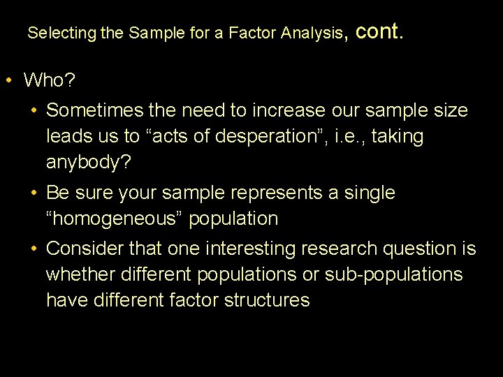
Selecting the Sample for a Factor Analysis, cont. • Who? • Sometimes the need to increase our sample size leads us to “acts of desperation”, i. e. , taking anybody? • Be sure your sample represents a single “homogeneous” population • Consider that one interesting research question is whether different populations or sub-populations have different factor structures