Principal Component Analysis Rotation into a new orthogonal

PCA: 2 variable example Weakly Correlated Variables Strongly Correlated Variables

Features of PCA ¡ ¡ ¡ EOFs must be mutually orthogonal; but physical modes

MOD EOF patterns and PC time series EOFs Var. (Cumul. Var. ) 42% 33%

MOD EOF 1: QBO (and Decadal) ¡ R=0. 80 ( 1% ) Captures 42%

EOF 4: ENSO <= 0 R=0. 71 ( < 0. 1% ) Captures 3%

PCA revisited ¡ ¡ Eigenvectors (spatial patterns) can be thought of as empirically derived

NCEP Geopotential Height: 30 mb – 100 mb Layer thickness EOFs Cumul. Var PCs

Slides: 11

Download presentation

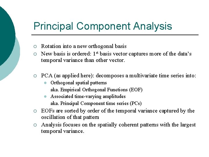
Principal Component Analysis ¡ Rotation into a new orthogonal basis New basis is ordered: 1 st basis vector captures more of the data’s temporal variance than other vector. ¡ PCA (as applied here): decomposes a multivariate time series into: ¡ l l ¡ ¡ Orthogonal spatial patterns aka. Empirical Orthogonal Functions (EOF) Associated time-varying amplitudes aka. Principal Component time series (PCs) EOFs are sorted by order of the temporal variance captured by the oscillation of that pattern Analysis focuses on the spatially coherent patterns with the largest temporal variance.

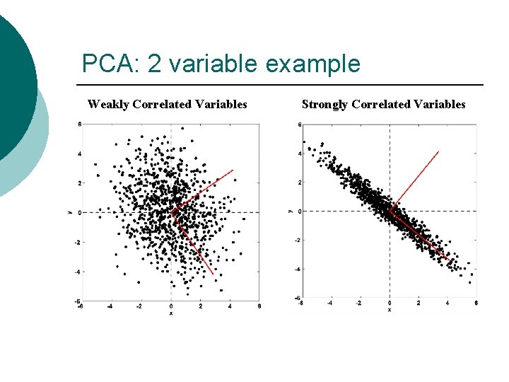
PCA: 2 variable example Weakly Correlated Variables Strongly Correlated Variables

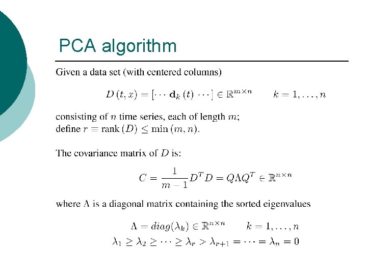
PCA algorithm

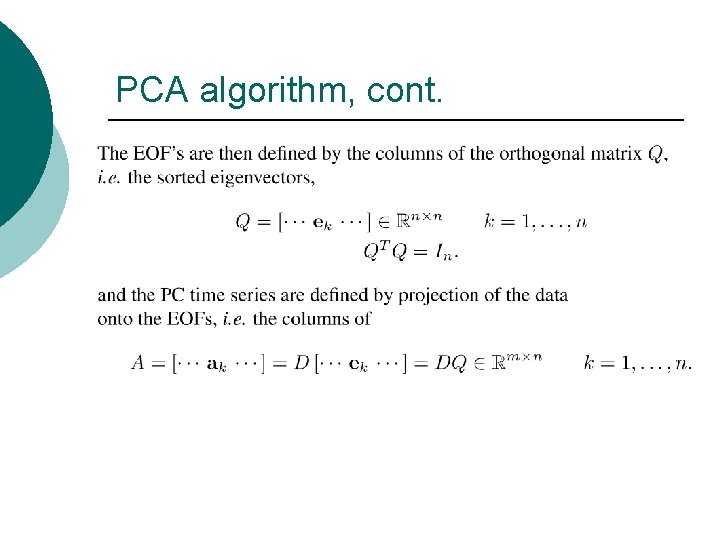
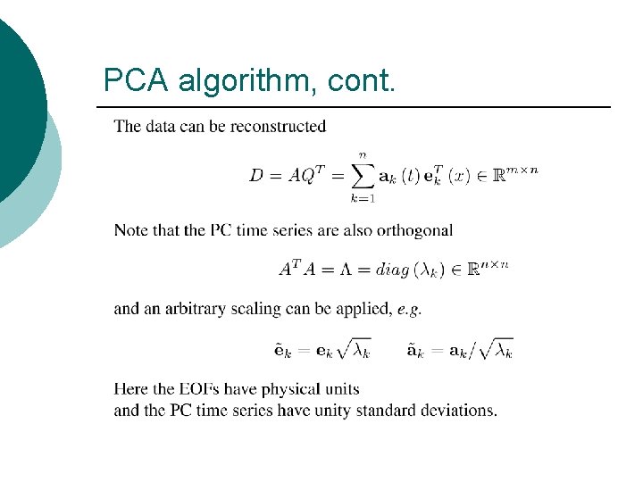
PCA algorithm, cont.

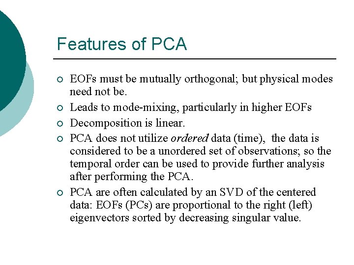
Features of PCA ¡ ¡ ¡ EOFs must be mutually orthogonal; but physical modes need not be. Leads to mode-mixing, particularly in higher EOFs Decomposition is linear. PCA does not utilize ordered data (time), the data is considered to be a unordered set of observations; so the temporal order can be used to provide further analysis after performing the PCA are often calculated by an SVD of the centered data: EOFs (PCs) are proportional to the right (left) eigenvectors sorted by decreasingular value.

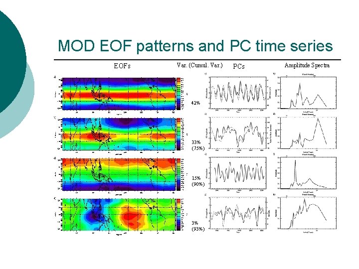
MOD EOF patterns and PC time series EOFs Var. (Cumul. Var. ) 42% 33% (75%) 15% (90%) 3% (93%) PCs Amplitude Spectra

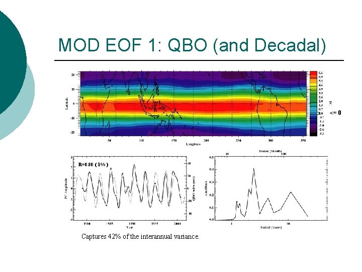
MOD EOF 1: QBO (and Decadal) ¡ R=0. 80 ( 1% ) Captures 42% of the interannual variance. <= 0

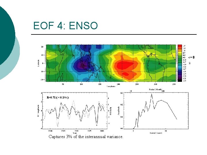
EOF 4: ENSO <= 0 R=0. 71 ( < 0. 1% ) Captures 3% of the interannual variance.

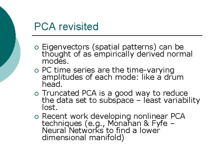
PCA revisited ¡ ¡ Eigenvectors (spatial patterns) can be thought of as empirically derived normal modes. PC time series are the time-varying amplitudes of each mode: like a drum head. Truncated PCA is a good way to reduce the data set to subspace – least variability lost. Recent work developing nonlinear PCA techniques (e. g. , Monahan & Fyfe – Neural Networks to find a lower dimensional manifold)

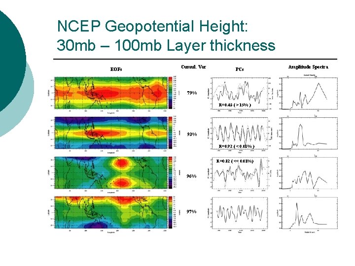
NCEP Geopotential Height: 30 mb – 100 mb Layer thickness EOFs Cumul. Var PCs 79% R=0. 43 ( > 15% ) 93% R=0. 92 ( < 0. 01% ) R=0. 82 ( << 0. 01%) 96% 97% Amplitude Spectra