Principal Component Analysis Olympic Heptathlon Ch 13 Principal

Principal Component Analysis Olympic Heptathlon Ch. 13

Principal components • The Principal components method summarizes data by finding the major correlations in linear combinations of the obervations. – Little information lost in process, usually – Major application: Correlated variables are transformed into uncorrelated variables

Olympic Heptathlon Data • 7 events: Hurdles, Highjump, Shot, run 200 m, longjump, javelin, run 800 m – The scores for these events are all on different scales – A relatively high number could be good or bad depending on the event • 25 Olympic competitors

R Commands • Reorder the scores so that a high number means a good score – heptathlon$hurdles <max(heptathlon$hurdles) – heptathlon$hurdles • Hurdles, Run 200 m, Run 800 m requires reordering

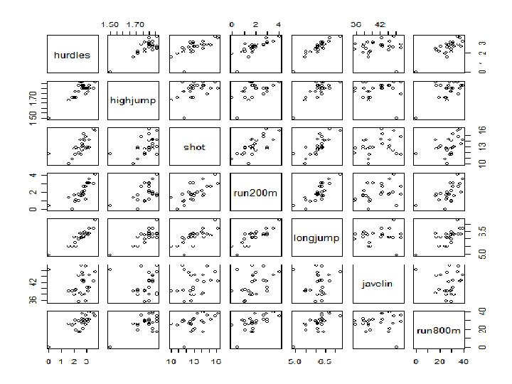
Basic plot to look at data • R Commands – score <- which(colnames(heptathlon) == “score”) • “which” searches the column names of the heptathlon data. frame for “score” and stores it in a variable “score” above – plot(heptathlon[, -score]) • Scatterplot matrix, excluding the score column

Interpretation • The data looks correlated except for the javelin event. – The book speculates the javelin is a ‘technical’ event, whereas the others are all ‘power’ events

To get numerical correlation values: • round(cor(heptathlon[, -score]), 2) • The cor(data. frame) function finds the actual correlation values • The cor(data. frame) function is in agreement with this interpretation hurdles 1. 00 highjump 0. 81 shot 0. 65 run 200 m 0. 77 longjump 0. 91 javelin 0. 01 run 800 m 0. 78 highjump 0. 81 1. 00 0. 44 0. 49 0. 78 0. 00 0. 59 shot run 200 m 0. 65 0. 77 0. 44 0. 49 1. 00 0. 68 1. 00 0. 74 0. 82 0. 27 0. 33 0. 42 0. 62 longjump 0. 91 0. 78 0. 74 0. 82 1. 00 0. 07 0. 70 javelin 0. 01 0. 00 0. 27 0. 33 0. 07 1. 00 -0. 02 run 800 m 0. 78 0. 59 0. 42 0. 62 0. 70 -0. 02 1. 00

Running a Principal Component analysis • heptathlon_pca <- prcomp(heptathlon[, -score], scale = TRUE) • print(heptathlon_pca) Standard deviations: [1] 2. 1119364 1. 0928497 0. 7218131 0. 6761411 0. 4952441 0. 2701029 0. 2213617 Rotation: PC 1 PC 2 PC 3 PC 4 PC 5 PC 6 PC 7 hurdles -0. 4528710 0. 15792058 -0. 04514996 0. 02653873 -0. 09494792 -0. 78334101 0. 38024707 highjump -0. 3771992 0. 24807386 -0. 36777902 0. 67999172 0. 01879888 0. 09939981 -0. 43393114 shot -0. 3630725 -0. 28940743 0. 67618919 0. 12431725 0. 51165201 -0. 05085983 -0. 21762491 run 200 m -0. 4078950 -0. 26038545 0. 08359211 -0. 36106580 -0. 64983404 0. 02495639 -0. 45338483 longjump -0. 4562318 0. 05587394 0. 13931653 0. 11129249 -0. 18429810 0. 59020972 0. 61206388 javelin -0. 0754090 -0. 84169212 -0. 47156016 0. 12079924 0. 13510669 -0. 02724076 0. 17294667 run 800 m -0. 3749594 0. 22448984 -0. 39585671 -0. 60341130 0. 50432116 0. 15555520 -0. 09830963

• a 1 <- heptathlon_pca$rotation[, 1] • a 1 • This shows the coefficients for the first principal component y 1 • Y 1 is the linear combination of observations that maximizes the sample variance as a portion of the overall sample variance. • Y 2 is the linear combination that maximizes out of the remaining portion of sample variance, with the added constraint of being uncorrelated with Y 1

• > a 1<-heptathlon_pca$rotation[, 1] • > a 1 hurdles highjump shot run 200 m longjump javelin run 800 m -0. 4528710 -0. 3771992 -0. 3630725 -0. 4078950 -0. 4562318 -0. 0754090 -0. 3749594

Interpretation • 200 m and long jump is the most important factor • Javelin result is less important

Data Analysis using the first principal component • center <- heptathlon_pca$center – This is the center or mean of the variables, it can also be a flag in the prcomp() function that sets the center at 0. • scale <- heptathlon_pca$scale – This is also a flag in the prcomp() function that can scale the variables to fit between 0 and 1, as it is, its just storing the current scale. – hm <- as. matrix(heptathlon[, -score]) • This coerces the data. frame heptathlon into a matrix and excludes score – drop(scale(hm, center = center, scale = scale) %*% heptathlon_pca$rotation[, 1]) • rescales the raw heptathlon data to the Principal component scale • performs matrix multiplication on the coefficients of the linear combination for the first principal component (Y 1) • Drop() prints the resulting matrix

Joyner-Kersee (USA) John (GDR) Behmer (GDR) Sablovskaite (URS) -4. 121447626 -2. 882185935 -2. 649633766 -1. 343351210 Choubenkova (URS) Schulz (GDR) Fleming (AUS) Greiner (USA) -1. 359025696 -1. 043847471 -1. 100385639 -0. 923173639 Lajbnerova (CZE) Bouraga (URS) Wijnsma (HOL) Dimitrova (BUL) -0. 530250689 -0. 759819024 -0. 556268302 -1. 186453832 Scheider (SWI) Braun (FRG) Ruotsalainen (FIN) Yuping (CHN) 0. 015461226 0. 003774223 0. 090747709 -0. 137225440 Hagger (GB) Brown (USA) Mulliner (GB) Hautenauve (BEL) 0. 171128651 0. 519252646 1. 125481833 1. 085697646 Kytola (FIN) Geremias (BRA) Hui-Ing (TAI) Jeong-Mi (KOR) 1. 447055499 2. 014029620 2. 880298635 2. 970118607 Launa (PNG) 6. 270021972

An easier way • predict(heptathlon_pca)[, 1] – Accomplishes the same thing as the previous set of commands

Principal Components Proportion of Sample Variances • The first component contributes the vast majority of total sample variance – Just looking at the first two (uncorrelated!) principal components will account for most of the overall sample variance (~81%) • plot(heptathlon_pca)

First two Principal Components biplot(heptathlon_pca, col=c("gray", "black"))

Interpretation • The Olympians with the highest score seem to be at the bottom left of the graph, while • The javelin event seems to give the scores a more fine variation and award the competitors a slight edge.

How well does it fit the Scoring? • The correlation between Y 1 and the scoring looks very strong. • cor(heptathlon$score, heptathlon_pca$x[, 1]) – [1] -0. 9910978

Homework! (Ch. 13) • Use the “meteo” data on page 225 and create scatterplots to check for correlation (don’t recode/reorder anything, and remember not to include columns in the analysis that don’t belong! – Is there correlation? Don’t have R calculate the numerical values unless you really want to • Run PCA using the long way or the shorter “predict” command (remember not to include the unneccesary column!) • Create a biplot, but use colors other than gray and black! • Create a scatterplot like on page 224 of the 1 st principle component and the yield – What is the numerical value of the correlation? • Don’t forget to copy and paste your commands into word and print it out for me (and include the scatterplot)!