Principal Component Analysis Jana Ludolph Martin Pokorny University

Principal Component Analysis Jana Ludolph Martin Pokorny University of Joensuu Dept. of Computer Science P. O. Box 111 FIN- 80101 Joensuu Tel. +358 13 251 7959 fax +358 13 251 7955 www. cs. joensuu. fi

PCA overview • Method objectives • Data dimensionality reduction • Clustering • Extract variables which properties are constitutive • Dimension reduction with minimal loss of information • History: – Pearson 1901 – Established 1930 Harold Hotelling – Since 1970 actually used (high perfomance computer) • Application: – Face recognition – Image processing – Artificial intelligence (neural network) • This material is PPT form of [1] with some changes University of Joensuu Dept. of Computer Science P. O. Box 111 FIN- 80101 Joensuu Tel. +358 13 251 7959 fax +358 13 251 7955 www. cs. joensuu. fi

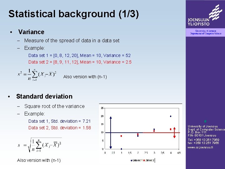
Statistical background (1/3) • Variance – Measure of the spread of data in a data set – Example: Data set 1 = [0, 8, 12, 20], Mean = 10, Variance = 52 Data set 2 = [8, 9, 11, 12], Mean = 10, Variance = 2. 5 Also version with (n-1) • Standard deviation – Square root of the variance – Example: Data set 1, Std. deviation = 7. 21 Data set 2, Std. deviation = 1. 58 Also version with (n-1) University of Joensuu Dept. of Computer Science P. O. Box 111 FIN- 80101 Joensuu Tel. +358 13 251 7959 fax +358 13 251 7955 www. cs. joensuu. fi

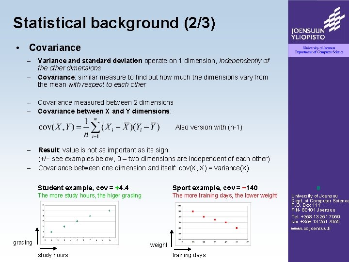
Statistical background (2/3) • Covariance – – Variance and standard deviation operate on 1 dimension, independently of the other dimensions Covariance: similar measure to find out how much the dimensions vary from the mean with respect to each other Covariance measured between 2 dimensions Covariance between X and Y dimensions: Also version with (n-1) – – Result: value is not as important as its sign (+/− see examples below, 0 – two dimensions are independent of each other) Covariance between one dimension and itself: cov(X, X) = variance(X) Student example, cov = +4. 4 Sport example, cov = − 140 The more study hours, the higer grading The more training days, the lower weight grading weight study hours training days University of Joensuu Dept. of Computer Science P. O. Box 111 FIN- 80101 Joensuu Tel. +358 13 251 7959 fax +358 13 251 7955 www. cs. joensuu. fi

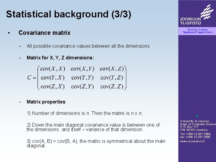
Statistical background (3/3) • Covariance matrix – All possible covariance values between all the dimensions – Matrix for X, Y, Z dimensions: – Matrix properties 1) Number of dimensions is n. Then the matrix is n x n. 2) Down the main diagonal covariance value is between one of the dimensions and itself – variance of that dimension. 3) cov(A, B) = cov(B, A), the matrix is symmetrical about the main diagonal. University of Joensuu Dept. of Computer Science P. O. Box 111 FIN- 80101 Joensuu Tel. +358 13 251 7959 fax +358 13 251 7955 www. cs. joensuu. fi

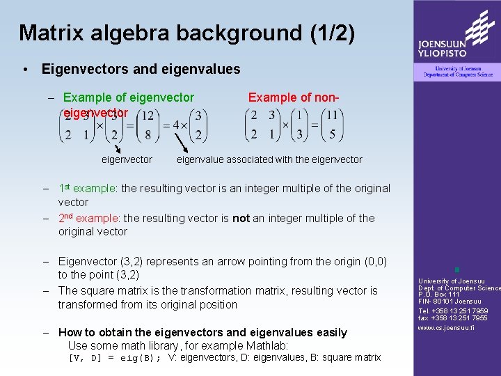
Matrix algebra background (1/2) • Eigenvectors and eigenvalues – Example of eigenvector Example of non- eigenvalue associated with the eigenvector – 1 st example: the resulting vector is an integer multiple of the original vector – 2 nd example: the resulting vector is not an integer multiple of the original vector – Eigenvector (3, 2) represents an arrow pointing from the origin (0, 0) to the point (3, 2) – The square matrix is the transformation matrix, resulting vector is transformed from its original position – How to obtain the eigenvectors and eigenvalues easily Use some math library, for example Mathlab: [V, D] = eig(B); V: eigenvectors, D: eigenvalues, B: square matrix University of Joensuu Dept. of Computer Science P. O. Box 111 FIN- 80101 Joensuu Tel. +358 13 251 7959 fax +358 13 251 7955 www. cs. joensuu. fi

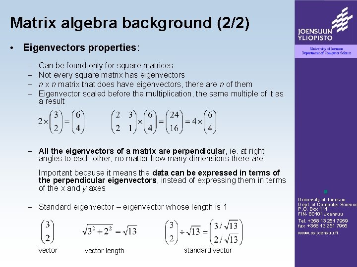
Matrix algebra background (2/2) • Eigenvectors properties: – – Can be found only for square matrices Not every square matrix has eigenvectors n x n matrix that does have eigenvectors, there are n of them Eigenvector scaled before the multiplication, the same multiple of it as a result – All the eigenvectors of a matrix are perpendicular, ie. at right angles to each other, no matter how many dimensions there are Important because it means the data can be expressed in terms of the perpendicular eigenvectors, instead of expressing them in terms of the x and y axes – Standard eigenvector – eigenvector whose length is 1 vector length standard vector University of Joensuu Dept. of Computer Science P. O. Box 111 FIN- 80101 Joensuu Tel. +358 13 251 7959 fax +358 13 251 7955 www. cs. joensuu. fi

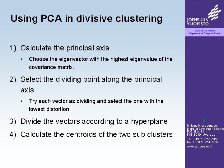
Using PCA in divisive clustering 1) Calculate the principal axis • Choose the eigenvector with the highest eigenvalue of the covariance matrix. 2) Select the dividing point along the principal axis • Try each vector as dividing and select the one with the lowest distortion. 3) Divide the vectors according to a hyperplane 4) Calculate the centroids of the two sub clusters University of Joensuu Dept. of Computer Science P. O. Box 111 FIN- 80101 Joensuu Tel. +358 13 251 7959 fax +358 13 251 7955 www. cs. joensuu. fi

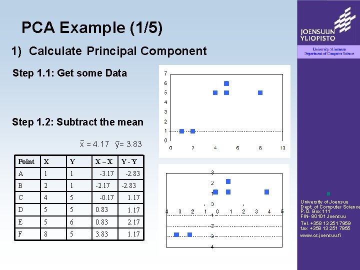
PCA Example (1/5) 1) Calculate Principal Component Step 1. 1: Get some Data Step 1. 2: Subtract the mean x = 4. 17 y= 3. 83 Point X Y X–X A 1 1 -3. 17 B 2 1 C 4 5 D 5 5 0. 83 1. 17 E 5 6 0. 83 2. 17 F 8 5 3. 83 1. 17 -2. 17 -0. 17 Y-Y -2. 83 1. 17 University of Joensuu Dept. of Computer Science P. O. Box 111 FIN- 80101 Joensuu Tel. +358 13 251 7959 fax +358 13 251 7955 www. cs. joensuu. fi

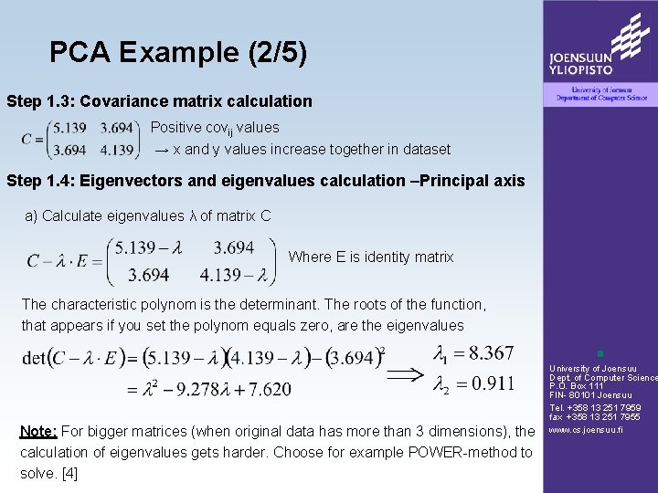
PCA Example (2/5) Step 1. 3: Covariance matrix calculation Positive covij values → x and y values increase together in dataset Step 1. 4: Eigenvectors and eigenvalues calculation –Principal axis a) Calculate eigenvalues λ of matrix C Where E is identity matrix The characteristic polynom is the determinant. The roots of the function, that appears if you set the polynom equals zero, are the eigenvalues Note: For bigger matrices (when original data has more than 3 dimensions), the calculation of eigenvalues gets harder. Choose for example POWER-method to solve. [4] University of Joensuu Dept. of Computer Science P. O. Box 111 FIN- 80101 Joensuu Tel. +358 13 251 7959 fax +358 13 251 7955 www. cs. joensuu. fi

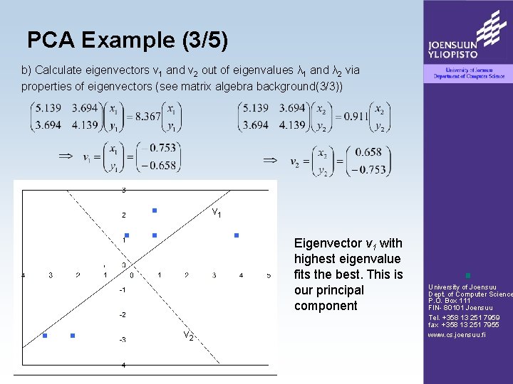
PCA Example (3/5) b) Calculate eigenvectors v 1 and v 2 out of eigenvalues λ 1 and λ 2 via properties of eigenvectors (see matrix algebra background(3/3)) v 1 Eigenvector v 1 with highest eigenvalue fits the best. This is our principal component v 2 University of Joensuu Dept. of Computer Science P. O. Box 111 FIN- 80101 Joensuu Tel. +358 13 251 7959 fax +358 13 251 7955 www. cs. joensuu. fi

PCA Example (4/5) 2) Select the dividig point along the principal axis Step 2. 1: Calculate projections on principal axis 2. 2 Sort according to their projections University of Joensuu Dept. of Computer Science P. O. Box 111 FIN- 80101 Joensuu Tel. +358 13 251 7959 fax +358 13 251 7955 www. cs. joensuu. fi

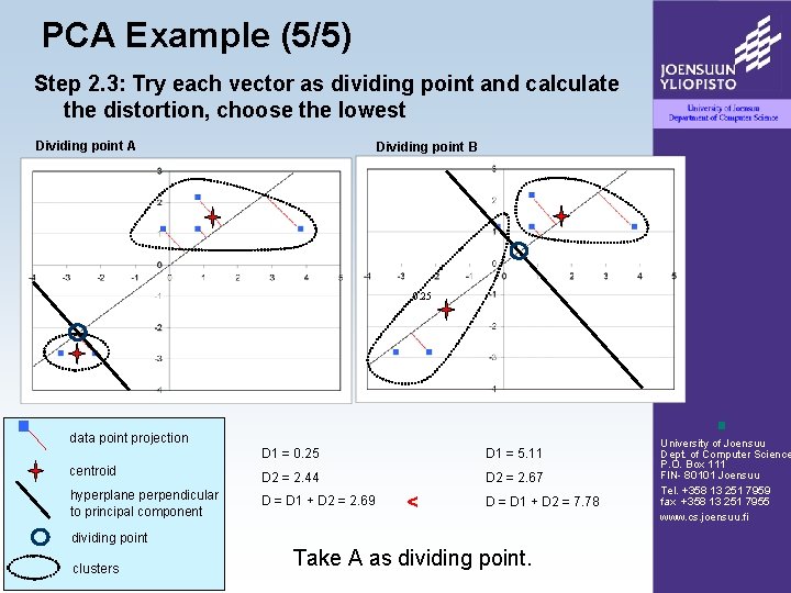
PCA Example (5/5) Step 2. 3: Try each vector as dividing point and calculate the distortion, choose the lowest Dividing point A Dividing point B 0. 25 data point projection D 1 = 0. 25 D 1 = 5. 11 centroid D 2 = 2. 44 D 2 = 2. 67 hyperplane perpendicular to principal component D = D 1 + D 2 = 2. 69 < D = D 1 + D 2 = 7. 78 dividing point clusters Take A as dividing point. University of Joensuu Dept. of Computer Science P. O. Box 111 FIN- 80101 Joensuu Tel. +358 13 251 7959 fax +358 13 251 7955 www. cs. joensuu. fi

References [1] Smith I L. : A tutorial on Principal Components Analysis. Student tutorial. 2002. http: //csnet. otago. ac. nz/cosc 453/student_tutorials/principal_components. pd f. [2] http: //de. wikipedia. org/wiki/Hauptkomponentenanalyse [3] http: //de. wikipedia. org/wiki/Eigenvektor [4] R. L. Burden and J. D. Faires, Numerical Analysis (third edition). Prindle, Weber & Smith, Boston, 1985. (p. 457) University of Joensuu Dept. of Computer Science P. O. Box 111 FIN- 80101 Joensuu Tel. +358 13 251 7959 fax +358 13 251 7955 www. cs. joensuu. fi