Principal Component Analysis Chapter 6 Feature extractionPCA Outline

Principal Component Analysis Chapter 6: Feature extraction_PCA

Outline • • Motivation Overview Intuitive approach Computation of PCA A Gaussian viewpoint Kernel PCA Exercise

Motivation • Question: What if the dimension of features we used is too high due to – Correlation between features – Not enough training samples(curse of dimensionality) • Solution: reduce the dimension of features by – Choosing some features that are most useful out – Deriving new low-dimension-features from the old one. (PCA can do this well)

Overview • Principal component analysis (PCA) is a way to reduce data dimensionality • PCA projects high dimensional data to a lower dimension • PCA projects the data in the least square error sense– it captures big (principal) variability in the data and ignores small variability

Intuitive approach • Let us say we have xi, i=1…N data points in p dimensions (p is large) • If we want to represent the data set by a single point x 0, then • Can we justify this choice mathematically? • It turns out that if you minimize J 0, you get the above solution

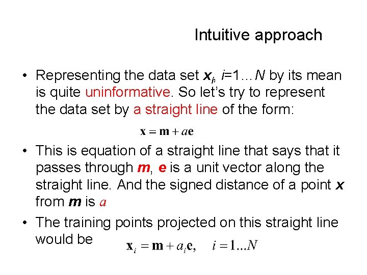
Intuitive approach • Representing the data set xi, i=1…N by its mean is quite uninformative. So let’s try to represent the data set by a straight line of the form: • This is equation of a straight line that says that it passes through m, e is a unit vector along the straight line. And the signed distance of a point x from m is a • The training points projected on this straight line would be

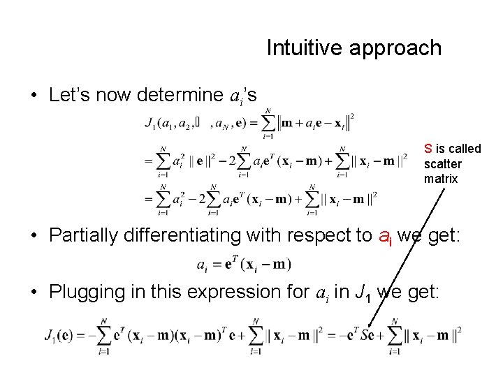
Intuitive approach • Let’s now determine ai’s S is called scatter matrix • Partially differentiating with respect to ai we get: • Plugging in this expression for ai in J 1 we get:

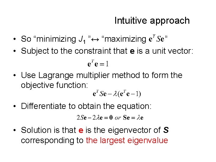
Intuitive approach • So “minimizing J 1 ”↔ “maximizing ” • Subject to the constraint that e is a unit vector: • Use Lagrange multiplier method to form the objective function: • Differentiate to obtain the equation: • Solution is that e is the eigenvector of S corresponding to the largest eigenvalue

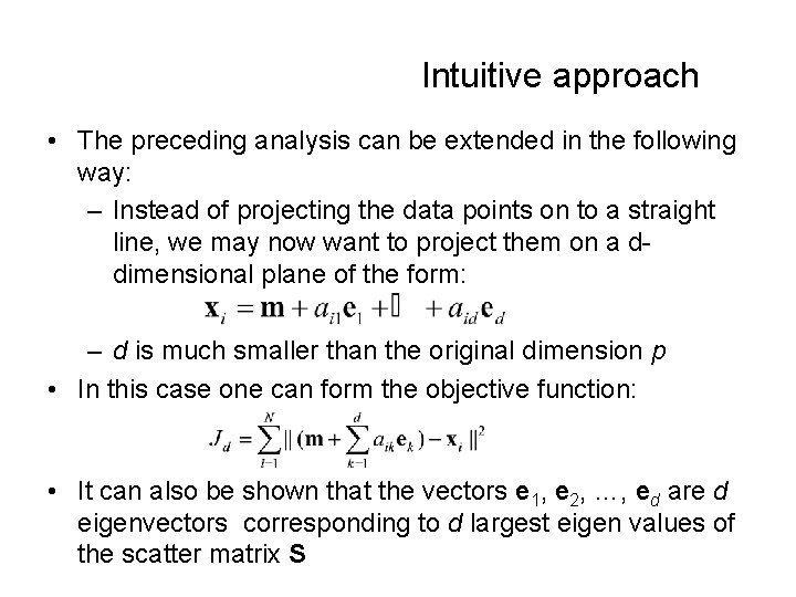
Intuitive approach • The preceding analysis can be extended in the following way: – Instead of projecting the data points on to a straight line, we may now want to project them on a ddimensional plane of the form: – d is much smaller than the original dimension p • In this case one can form the objective function: • It can also be shown that the vectors e 1, e 2, …, ed are d eigenvectors corresponding to d largest eigen values of the scatter matrix S

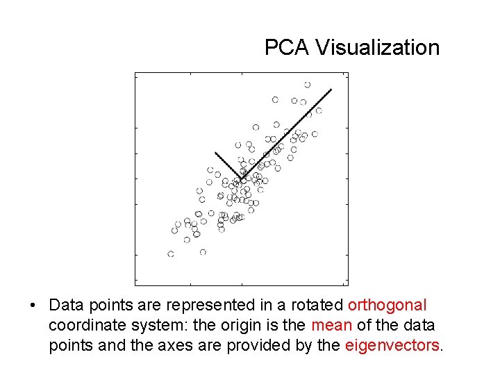
PCA Visualization • Data points are represented in a rotated orthogonal coordinate system: the origin is the mean of the data points and the axes are provided by the eigenvectors.

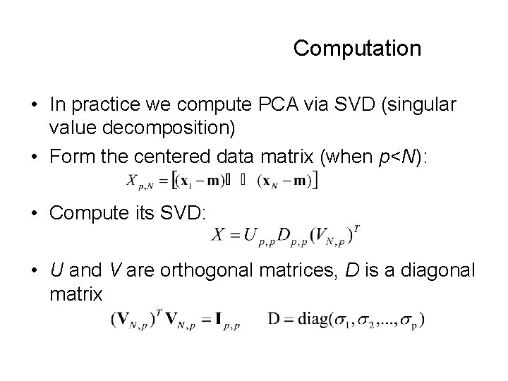
Computation • In practice we compute PCA via SVD (singular value decomposition) • Form the centered data matrix (when p<N): • Compute its SVD: • U and V are orthogonal matrices, D is a diagonal matrix

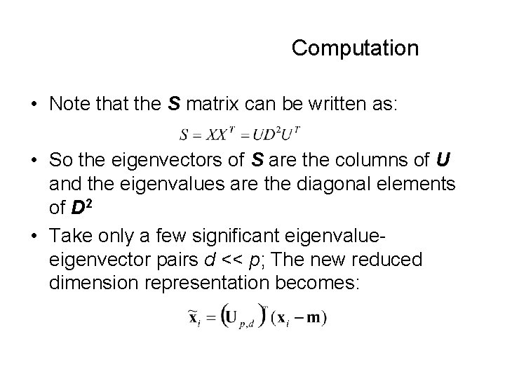
Computation • Note that the S matrix can be written as: • So the eigenvectors of S are the columns of U and the eigenvalues are the diagonal elements of D 2 • Take only a few significant eigenvalueeigenvector pairs d << p; The new reduced dimension representation becomes:

Computation • Sometimes we are given only a few high dimensional data points, i. e. , p >> N • In such cases compute the SVD of XT: • So that we get: • Then, proceed as before, choose only d < N significant eigenvalues for data representation:

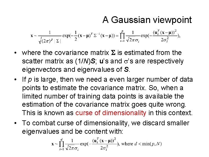
A Gaussian viewpoint • where the covariance matrix is estimated from the scatter matrix as (1/N)S; u’s and ’s are respectively eigenvectors and eigenvalues of S. • If p is large, then we need a even larger number of data points to estimate the covariance matrix. So, when a limited number of training data points is available the estimation of the covariance matrix goes quite wrong. This is known as curse of dimensionality in this context. • To combat curse of dimensionality, we discard smaller eigenvalues and be content with:

Kernel PCA • Assumption behind PCA is that the data points x are multivariate Gaussian • Often this assumption does not hold • However, it may still be possible that a transformation (x) is still Gaussian, then we can perform PCA in the space of (x) • Kernel PCA performs this PCA; however, because of “kernel trick, ” it never computes the mapping (x) explicitly!

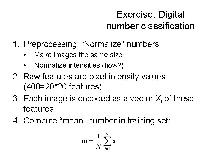
Exercise: Digital number classification 1. Preprocessing: “Normalize” numbers • • Make images the same size Normalize intensities (how? ) 2. Raw features are pixel intensity values (400=20*20 features) 3. Each image is encoded as a vector Xi of these features 4. Compute “mean” number in training set:

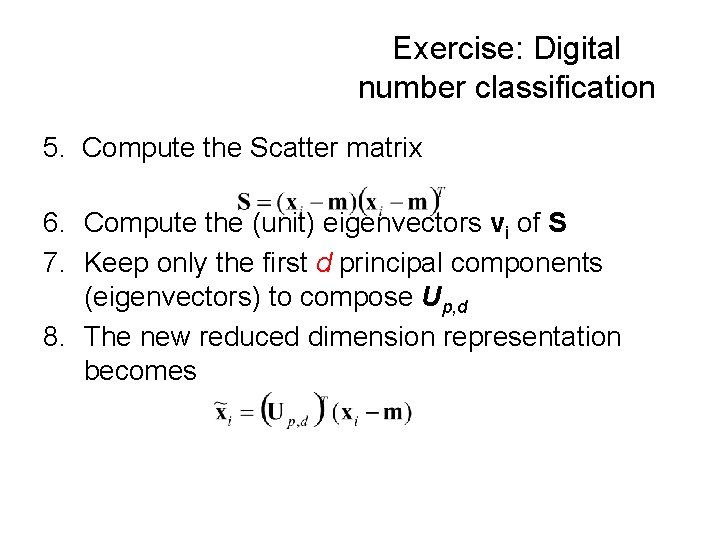
Exercise: Digital number classification 5. Compute the Scatter matrix 6. Compute the (unit) eigenvectors vi of S 7. Keep only the first d principal components (eigenvectors) to compose Up, d 8. The new reduced dimension representation becomes

Exercise: Digital number classification • The eigen-numbers encode the principal sources of variation in the dataset ( try to find some real meanings by show these eigen-numbers as images like eigenfaces!). • We can represent any number as a linear combination of these “basis” numbers. (show me!) • Use this new representation for: • – Number recognition (e. g. , MED classifier and MICD classifier of number) “numbers” versus “no numbers” need “no number” training samples.