Principal Component Analysis Biosystems Data Analysis UNIVERSITY OF

Principal Component Analysis Biosystems Data Analysis UNIVERSITY OF A MSTERDAM 1

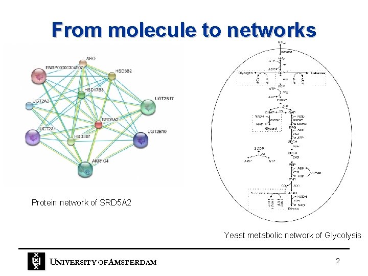
From molecule to networks Protein network of SRD 5 A 2 Yeast metabolic network of Glycolysis UNIVERSITY OF A MSTERDAM 2

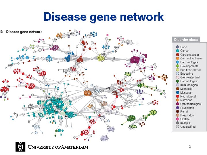
Disease gene network UNIVERSITY OF A MSTERDAM 3

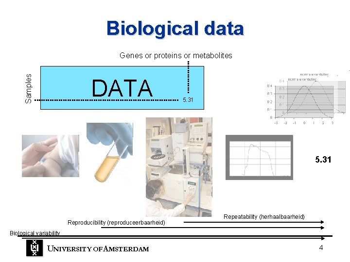
Biological data Samples Genes or proteins or metabolites DATA 5. 31 Reproducibility (reproduceerbaarheid) Repeatability (herhaalbaarheid) Biological variability UNIVERSITY OF A MSTERDAM 4

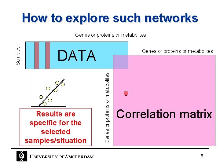
How to explore such networks DATA Results are specific for the selected samples/situation UNIVERSITY OF A MSTERDAM Genes or proteins or metabolites Samples Genes or proteins or metabolites Correlation matrix 5

Goals • If you measure multiple variables on an object it can be important to analyze the measurements simultaneously. • Understand the most important tool in multivariate data analysis Principal Component Analysis. UNIVERSITY OF A MSTERDAM 6

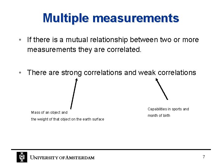
Multiple measurements • If there is a mutual relationship between two or more measurements they are correlated. • There are strong correlations and weak correlations Mass of an object and the weight of that object on the earth surface UNIVERSITY OF A MSTERDAM Capabilities in sports and month of birth 7

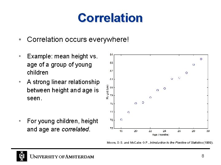
Correlation • Correlation occurs everywhere! • Example: mean height vs. age of a group of young children • A strong linear relationship between height and age is seen. • For young children, height and age are correlated. Moore, D. S. and Mc. Cabe G. P. , Introduction to the Practice of Statistics (1989). UNIVERSITY OF A MSTERDAM 8

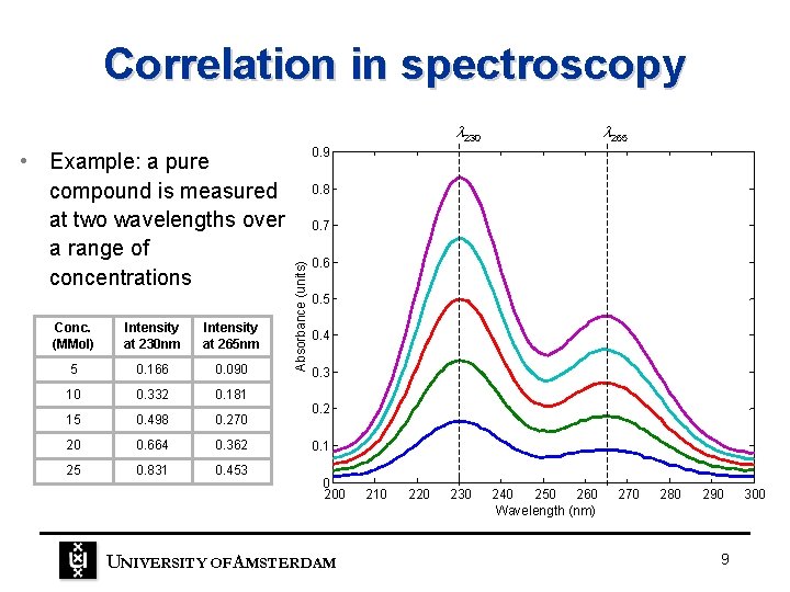
Correlation in spectroscopy 230 Conc. (MMol) Intensity at 230 nm Intensity at 265 nm 5 0. 166 0. 090 10 0. 332 0. 181 15 0. 498 0. 270 20 0. 664 0. 362 25 0. 831 0. 453 0. 9 0. 8 0. 7 Absorbance (units) • Example: a pure compound is measured at two wavelengths over a range of concentrations 265 0. 6 0. 5 0. 4 0. 3 0. 2 0. 1 0 200 UNIVERSITY OF A MSTERDAM 210 220 230 240 250 260 Wavelength (nm) 270 280 290 9 300

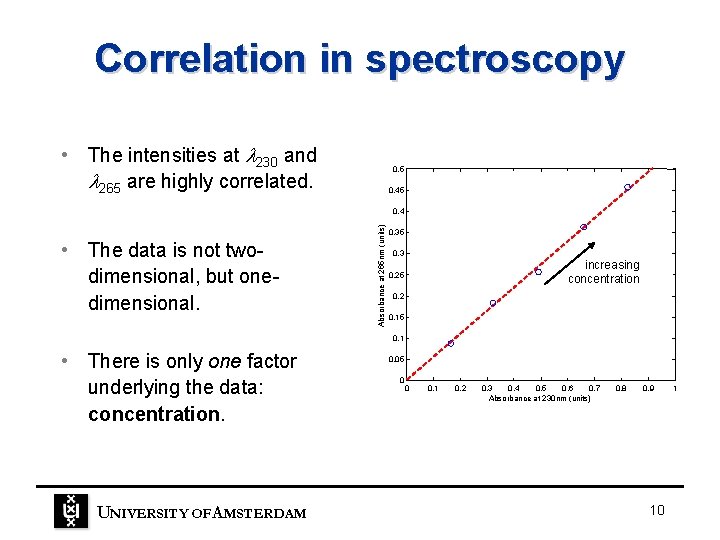
Correlation in spectroscopy • The intensities at 230 and 265 are highly correlated. 0. 5 0. 45 • The data is not twodimensional, but onedimensional. Absorbance at 265 nm (units) 0. 4 0. 35 0. 3 increasing concentration 0. 25 0. 2 0. 15 0. 1 • There is only one factor underlying the data: concentration. UNIVERSITY OF A MSTERDAM 0. 05 0 0 0. 1 0. 2 0. 3 0. 4 0. 5 0. 6 0. 7 Absorbance at 230 nm (units) 0. 8 0. 9 10 1

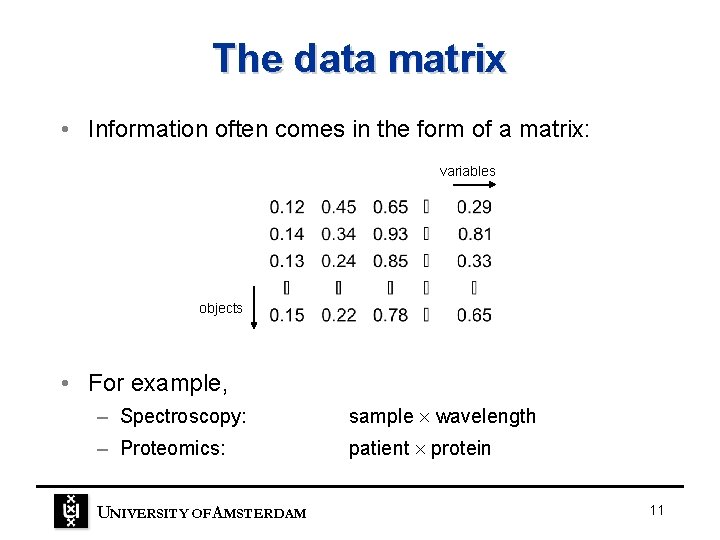
The data matrix • Information often comes in the form of a matrix: variables objects • For example, – Spectroscopy: sample wavelength – Proteomics: patient protein UNIVERSITY OF A MSTERDAM 11

Large amounts of data • In (bio)chemical analysis, the measured data matrices can be very large. – An infrared spectrum measured for 50 samples gives a data matrix of size 50 800 = 40, 000 numbers! – The matabolome of a 100 patient yield a data matrix of size 1000 = 100, 000 numbers. • We need a way of extracting the important information from large data matrices. UNIVERSITY OF A MSTERDAM 12

Principal Component Analysis • Data reduction – PCA reduces large data matrices into two smaller matrices which can be more easily examined, plotted and interpreted. • Data exploration – PCA extracts the most important factors (principal components) from the data. These factors describe multivariate interactions between the measured variables. • Data understanding – Principal components can be used to classify samples, identify compound spectra, determine biomarker etc. UNIVERSITY OF A MSTERDAM 13

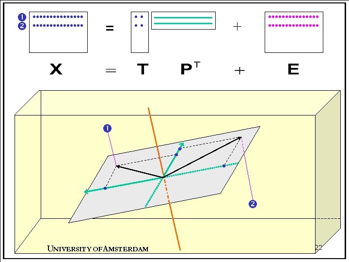
Different views of PCA • Statistically, PCA is a multivariate analysis technique closely related to – eigenvector analysis – singular value decomposition (SVD) • In matrix terms, PCA is a decomposition of X into two smaller matrices plus a set of residuals: X = TPT + E • Geometrically, PCA is a projection technique in which X is projected onto a subspace of reduced dimensions. UNIVERSITY OF A MSTERDAM 14

PCA: mathematics • The basic equation for PCA is written as where X (I J) is a data matrix, T (I R) are the scores, P (J R) are the loadings and E (I J) are the residuals. R is the number of principal components used to describe X. UNIVERSITY OF A MSTERDAM 15

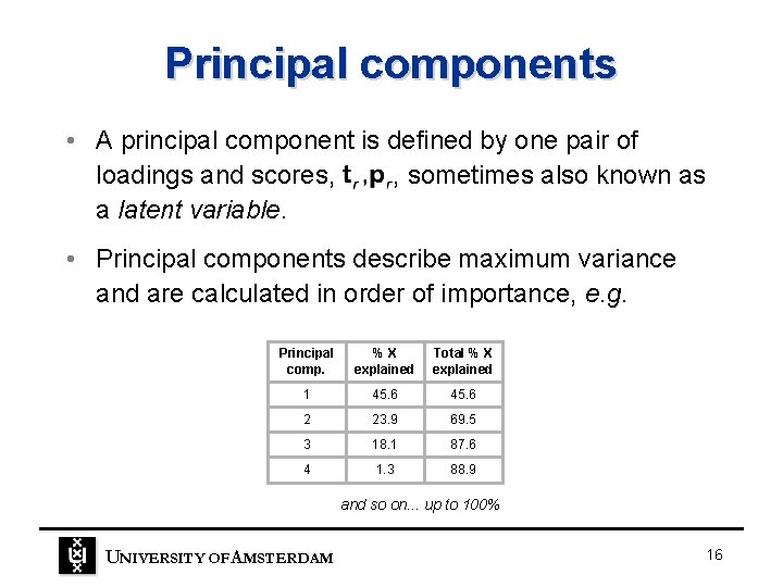
Principal components • A principal component is defined by one pair of loadings and scores, , sometimes also known as a latent variable. • Principal components describe maximum variance and are calculated in order of importance, e. g. Principal comp. %X explained Total % X explained 1 45. 6 2 23. 9 69. 5 3 18. 1 87. 6 4 1. 3 88. 9 and so on. . . up to 100% UNIVERSITY OF A MSTERDAM 16

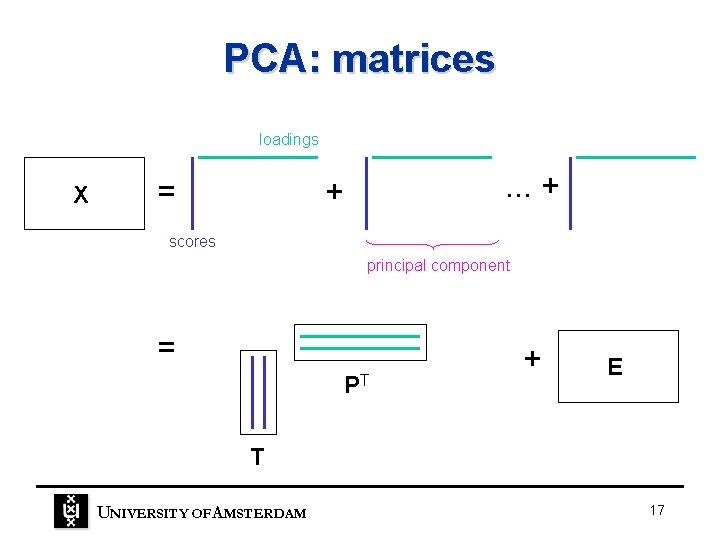
PCA: matrices loadings X = . . . + + scores principal component = PT + E T UNIVERSITY OF A MSTERDAM 17

Scores and loadings • Scores – relationships between objects – orthogonal, TTT = diagonal matrix • Loadings – relationships between variables – orthonormal, PTP = identity matrix, I • Similarities and differences between objects (or variables) can be seen by plotting scores (or loadings) against each other. UNIVERSITY OF A MSTERDAM 18

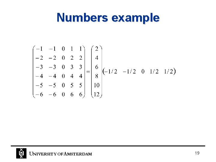
Numbers example UNIVERSITY OF A MSTERDAM 19

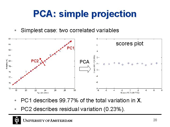
PCA: simple projection • Simplest case: two correlated variables scores plot PC 1 PC 2 PCA • PC 1 describes 99. 77% of the total variation in X. • PC 2 describes residual variation (0. 23%). UNIVERSITY OF A MSTERDAM 20

PCA: projections • PCA is a projection technique. • Each row of the data matrix X (I J) can be considered as a point in J-dimensional space. This data is projected orthogonally onto a subspace of lower dimensionality. – In the previous example, we projected the two-dimensional data onto a one-dimensional space, i. e. onto a line. – Now we will project some J-dimensional data onto a twodimensional space, i. e. onto a plane. UNIVERSITY OF A MSTERDAM 21

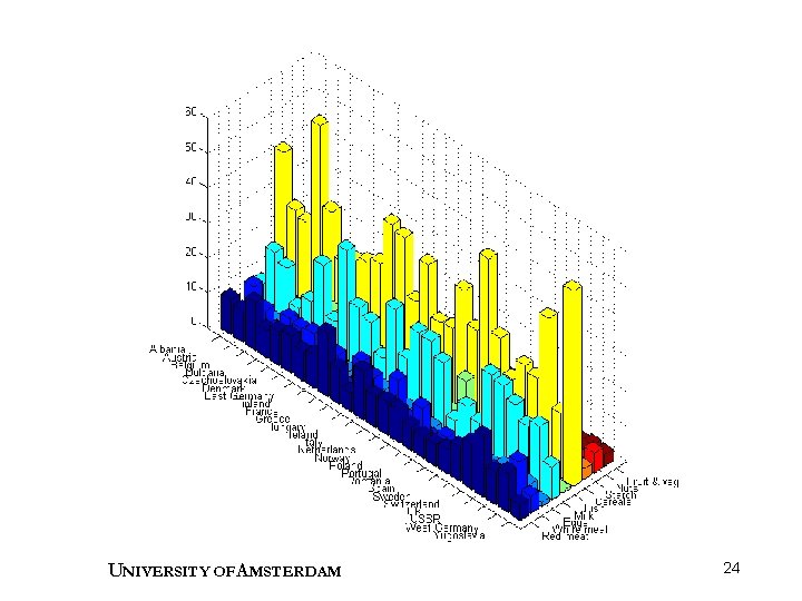
Example : Protein data • Protein consumption across Europe was studied. • 9 variables describe different sources of protein. • 25 objects are the different countries. • Data matrix has dimensions 25 9. • Which countries are similar? • Which foods are related to red meat consumption? Weber, A. , Agrarpolitik im Spannungsfeld der internationalen Ernaehrungspolitik, Institut fuer Agrarpolitik und marktlehre, Kiel (1973). UNIVERSITY OF A MSTERDAM 23

UNIVERSITY OF A MSTERDAM 24

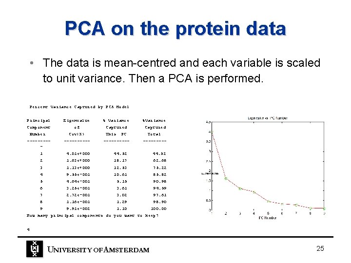
PCA on the protein data • The data is mean-centred and each variable is scaled to unit variance. Then a PCA is performed. Percent Variance Captured by PCA Model Principal Component Number Eigenvalue of Cov(X) ---------- % Variance %Variance Captured This PC ----- Total ----- 1 4. 01 e+000 44. 52 2 1. 63 e+000 18. 17 62. 68 3 1. 13 e+000 12. 53 75. 22 4 9. 55 e-001 10. 61 85. 82 5 4. 64 e-001 5. 15 90. 98 6 3. 25 e-001 3. 61 94. 59 7 2. 72 e-001 3. 02 97. 61 8 1. 16 e-001 1. 29 98. 90 9 9. 91 e-002 1. 10 100. 00 How many principal components do you want to keep? 4 UNIVERSITY OF A MSTERDAM 25

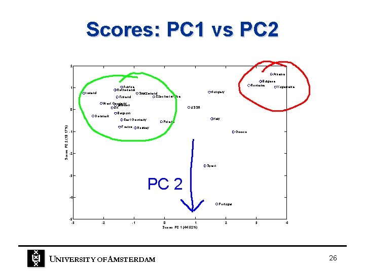
Scores: PC 1 vs PC 2 2 Albania Austria Netherlands 1 Ireland 0 Finland Hungary Switzerland Czechoslovakia West Germany Sweden UK Denmark Scores PC 2 (18. 17%) Bulgaria Romania Yugoslavia USSR Belgium East Germany France Poland Italy Norway -1 Greece -2 Spain -3 PC 2 -4 Portugal -5 -3 -2 -1 UNIVERSITY OF A MSTERDAM 0 1 Scores PC 1 (44. 52%) 2 3 4 26

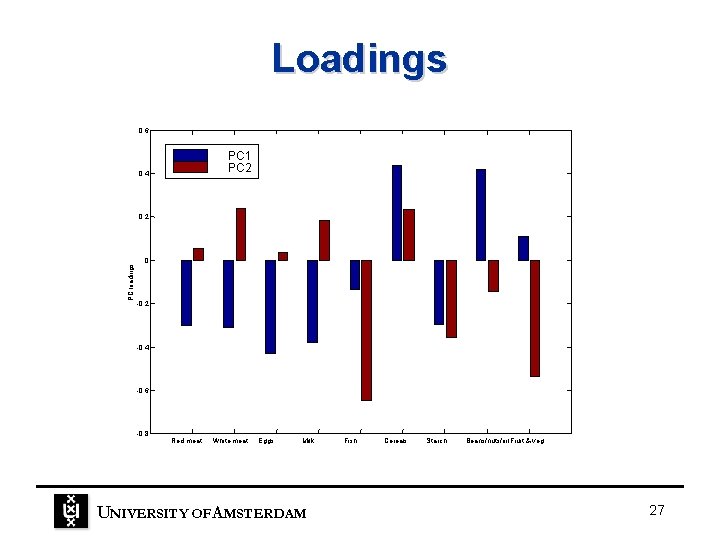
Loadings 0. 6 PC 1 PC 2 0. 4 PC loadings 0. 2 0 -0. 2 -0. 4 -0. 6 -0. 8 Red meat White meat Eggs Milk UNIVERSITY OF A MSTERDAM Fish Cereals Starch Beans/nuts/oil. Fruit & veg 27

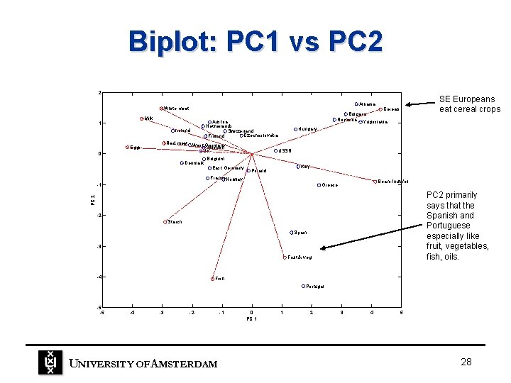
Biplot: PC 1 vs PC 2 2 Milk 1 Ireland 0 Denmark Cereals Bulgaria Romania Yugoslavia Austria Netherlands Switzerland Czechoslovakia Finland Red meat West Germany Sweden UK Eggs SE Europeans eat cereal crops Albania White meat Hungary USSR Belgium East Germany Italy Poland France. Norway Beans/nuts/oil Greece PC 2 primarily says that the Spanish and Portuguese especially like fruit, vegetables, fish, oils. PC 2 -1 -2 Starch Spain -3 Fruit & veg -4 Fish Portugal -5 -5 -4 -3 -2 UNIVERSITY OF A MSTERDAM -1 0 PC 1 1 2 3 4 5 28

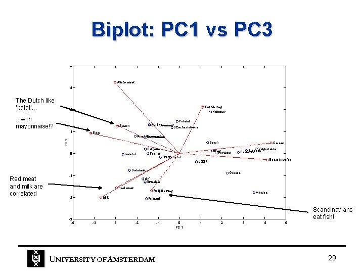
Biplot: PC 1 vs PC 3 4 White meat 3 The Dutch like ‘patat’. . . Fruit & veg Hungary 2 . . . with mayonnaise!? Poland Austria East Germany Czechoslovakia Starch Eggs West Germany Netherlands PC 3 1 Spain 0 Belgium France Ireland Cereals Italy Portugal Yugoslavia Bulgaria Romania Switzerland Beans/nuts/oil USSR Denmark Red meat and milk are correlated -1 Red meat -2 -3 -5 Greece UK Sweden Fish Norway Milk Albania Finland Scandinavians eat fish! -4 -3 -2 UNIVERSITY OF A MSTERDAM -1 0 PC 1 1 2 3 4 5 29

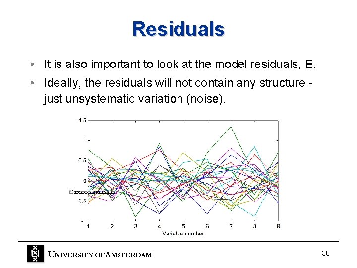
Residuals • It is also important to look at the model residuals, E. • Ideally, the residuals will not contain any structure just unsystematic variation (noise). UNIVERSITY OF A MSTERDAM 30

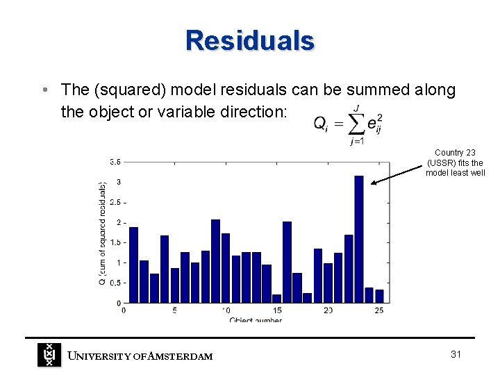
Residuals • The (squared) model residuals can be summed along the object or variable direction: Country 23 (USSR) fits the model least well UNIVERSITY OF A MSTERDAM 31

Centering and scaling • We are often interested in the differences between objects, not in their absolute values. – protein data: differences between countries • If different variables are measured in different units, some scaling is needed to give each variable an equal chance of contributing to the model. UNIVERSITY OF A MSTERDAM 32

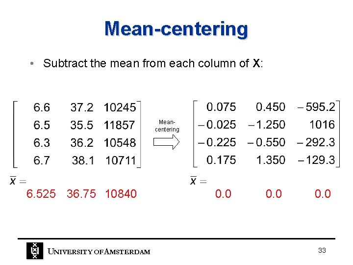
Mean-centering • Subtract the mean from each column of X: Meancentering 6. 525 36. 75 10840 UNIVERSITY OF A MSTERDAM 0. 0 33

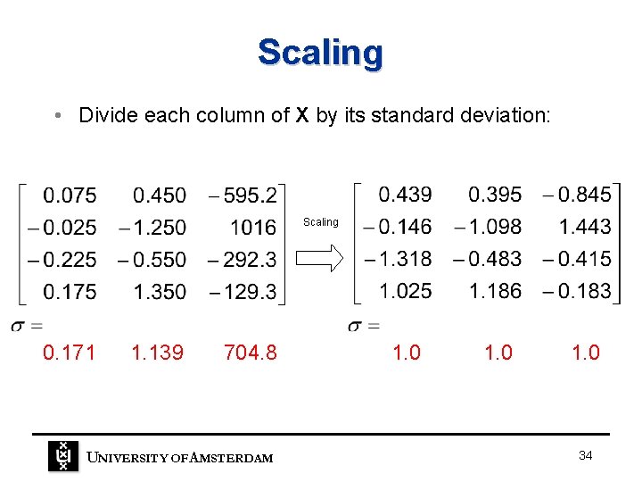
Scaling • Divide each column of X by its standard deviation: Scaling 0. 171 1. 139 704. 8 UNIVERSITY OF A MSTERDAM 1. 0 34

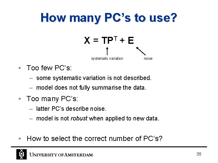
How many PC’s to use? X = TPT + E systematic variation noise • Too few PC’s: – some systematic variation is not described. – model does not fully summarise the data. • Too many PC’s: – latter PC’s describe noise. – model is not robust when applied to new data. • How to select the correct number of PC’s? UNIVERSITY OF A MSTERDAM 35

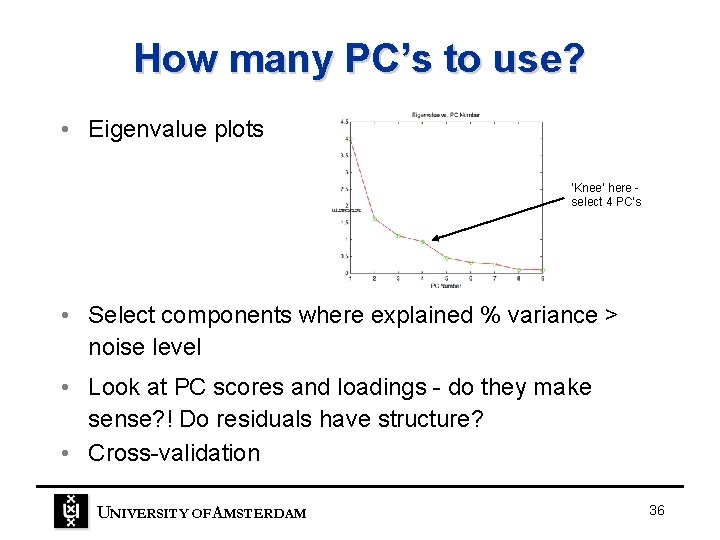
How many PC’s to use? • Eigenvalue plots ‘Knee’ here select 4 PC’s • Select components where explained % variance > noise level • Look at PC scores and loadings - do they make sense? ! Do residuals have structure? • Cross-validation UNIVERSITY OF A MSTERDAM 36

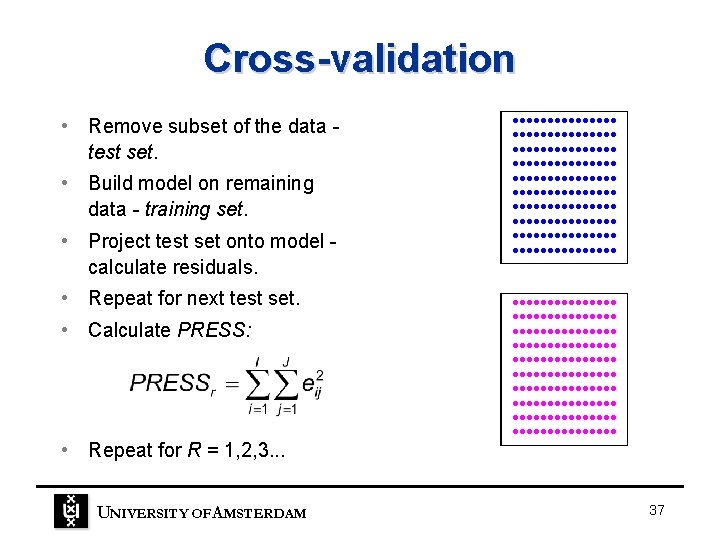
Cross-validation • Remove subset of the data test set. • Build model on remaining data - training set. • Project test set onto model calculate residuals. • Repeat for next test set. • Calculate PRESS: • Repeat for R = 1, 2, 3. . . UNIVERSITY OF A MSTERDAM • • • • • • • • • • • • • • • • • • • • • • • • • • • • • • • • • • • • • • • • • • • • • • • • • • • • • • • • • • • • • • • • • • • • • • • • • • • 37

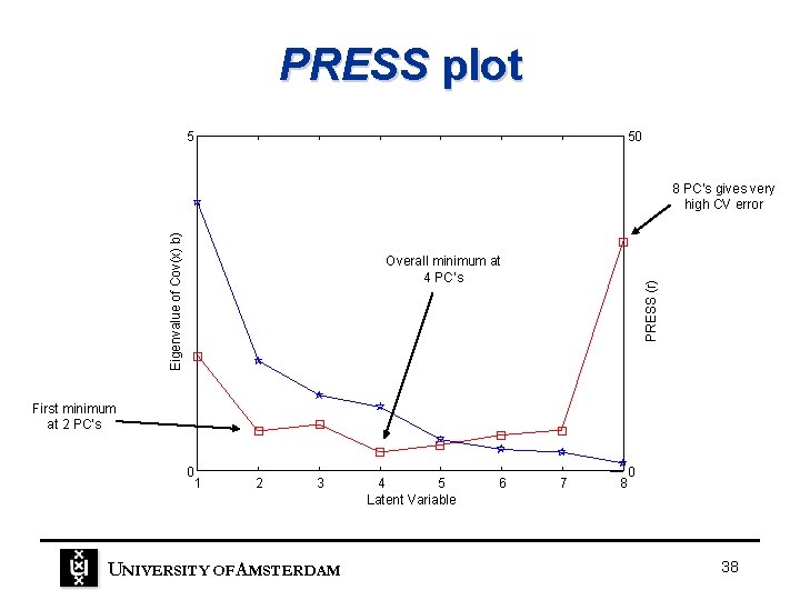
PRESS plot 5 50 Eigenvalue of Cov(x) b) 8 PC’s gives very high CV error PRESS (r) Overall minimum at 4 PC’s First minimum at 2 PC’s 0 1 2 3 UNIVERSITY OF A MSTERDAM 4 5 Latent Variable 6 7 0 8 38

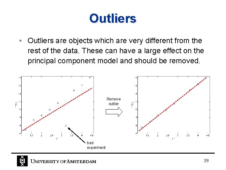
Outliers • Outliers are objects which are very different from the rest of the data. These can have a large effect on the principal component model and should be removed. Remove outlier bad experiment UNIVERSITY OF A MSTERDAM 39

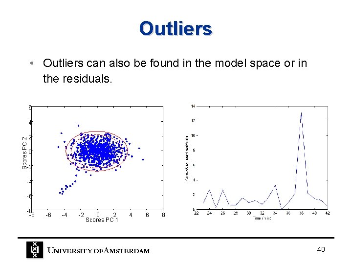
Outliers • Outliers can also be found in the model space or in the residuals. 6 Scores PC 2 4 2 0 -2 -4 -6 -8 -8 -6 -4 -2 0 2 Scores PC 1 4 6 UNIVERSITY OF A MSTERDAM 8 40

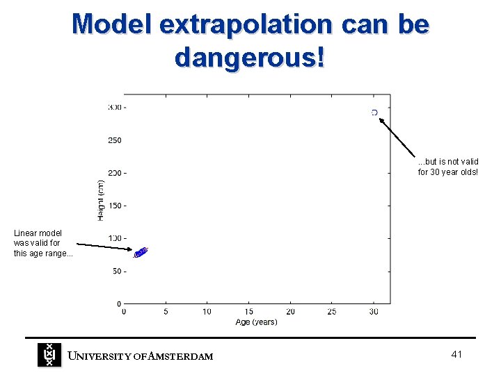
Model extrapolation can be dangerous! . . . but is not valid for 30 year olds! Linear model was valid for this age range. . . UNIVERSITY OF A MSTERDAM 41

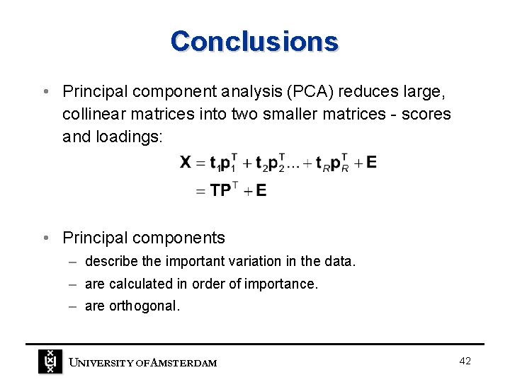
Conclusions • Principal component analysis (PCA) reduces large, collinear matrices into two smaller matrices - scores and loadings: • Principal components – describe the important variation in the data. – are calculated in order of importance. – are orthogonal. UNIVERSITY OF A MSTERDAM 42

Conclusions • Scores plots and biplots can be useful for exploring and understanding the data. • It is often correct to mean-center and scale the variables prior to analysis. • It is important to include the correct number of PC’s in the PCA model. One method for determining this is called cross-validation. UNIVERSITY OF A MSTERDAM 43