Principal Component Analysis and Independent Component Analysis in

Principal Component Analysis and Independent Component Analysis in Neural Networks David Gleich CS 152 – Neural Networks 6 November 2003

TLAs • • TLA – Three Letter Acronym PCA – Principal Component Analysis ICA – Independent Component Analysis SVD – Singular-Value Decomposition

Outline • Principal Component Analysis – Introduction – Linear Algebra Approach – Neural Network Implementation • Independent Component Analysis – Introduction – Demos – Neural Network Implementations • References • Questions

Principal Component Analysis • PCA identifies an m dimensional explanation of n dimensional data where m < n. • Originated as a statistical analysis technique. • PCA attempts to minimize the reconstruction error under the following restrictions – Linear Reconstruction – Orthogonal Factors • Equivalently, PCA attempts to maximize variance, proof coming.

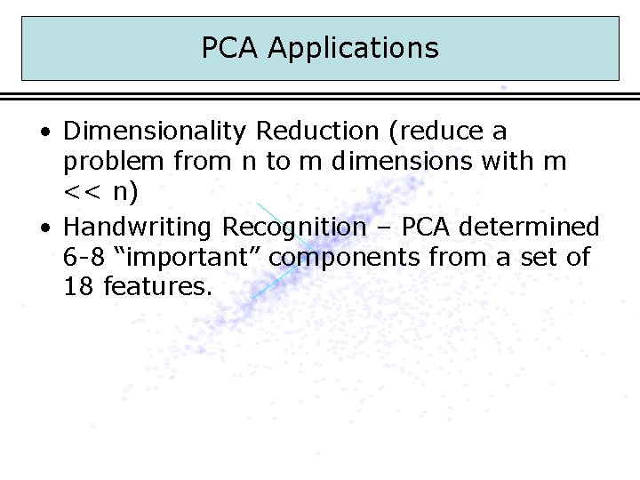
PCA Applications • Dimensionality Reduction (reduce a problem from n to m dimensions with m << n) • Handwriting Recognition – PCA determined 6 -8 “important” components from a set of 18 features.

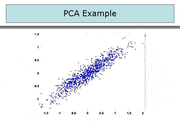
PCA Example

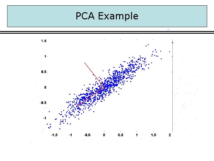
PCA Example

PCA Example

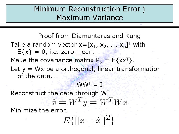
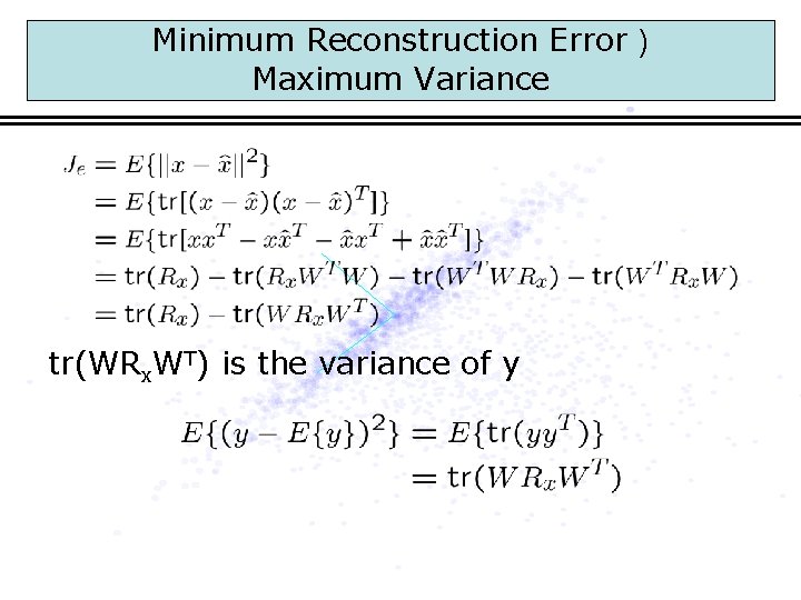
Minimum Reconstruction Error ) Maximum Variance Proof from Diamantaras and Kung Take a random vector x=[x 1, x 2, …, xn]T with E{x} = 0, i. e. zero mean. Make the covariance matrix Rx = E{xx. T}. Let y = Wx be a orthogonal, linear transformation of the data. WWT = I Reconstruct the data through WT. Minimize the error.

Minimum Reconstruction Error ) Maximum Variance tr(WRx. WT) is the variance of y

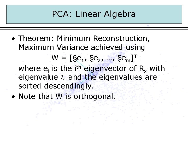
PCA: Linear Algebra • Theorem: Minimum Reconstruction, Maximum Variance achieved using W = [§e 1, §e 2, …, §em]T where ei is the ith eigenvector of Rx with eigenvalue i and the eigenvalues are sorted descendingly. • Note that W is orthogonal.

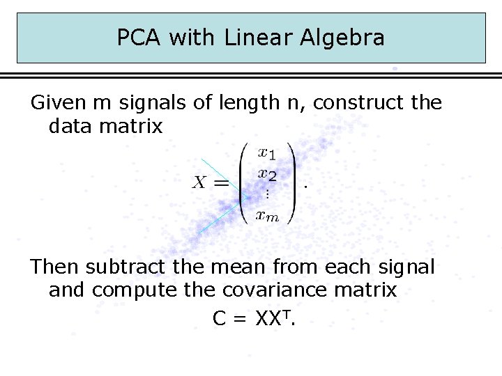
PCA with Linear Algebra Given m signals of length n, construct the data matrix Then subtract the mean from each signal and compute the covariance matrix C = XXT.

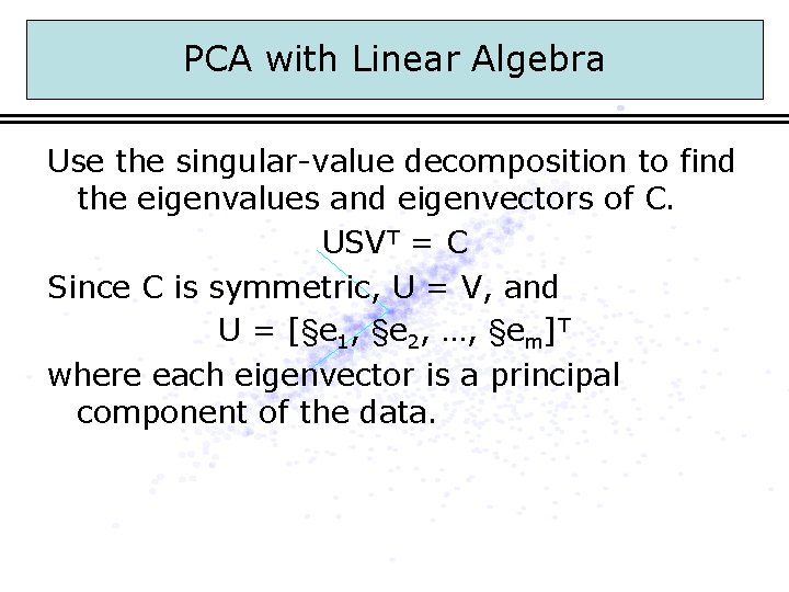
PCA with Linear Algebra Use the singular-value decomposition to find the eigenvalues and eigenvectors of C. USVT = C Since C is symmetric, U = V, and U = [§e 1, §e 2, …, §em]T where each eigenvector is a principal component of the data.

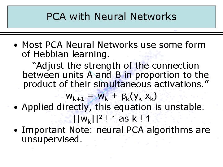
PCA with Neural Networks • Most PCA Neural Networks use some form of Hebbian learning. “Adjust the strength of the connection between units A and B in proportion to the product of their simultaneous activations. ” wk+1 = wk + k(yk xk) • Applied directly, this equation is unstable. ||wk||2 ! 1 as k ! 1 • Important Note: neural PCA algorithms are unsupervised.

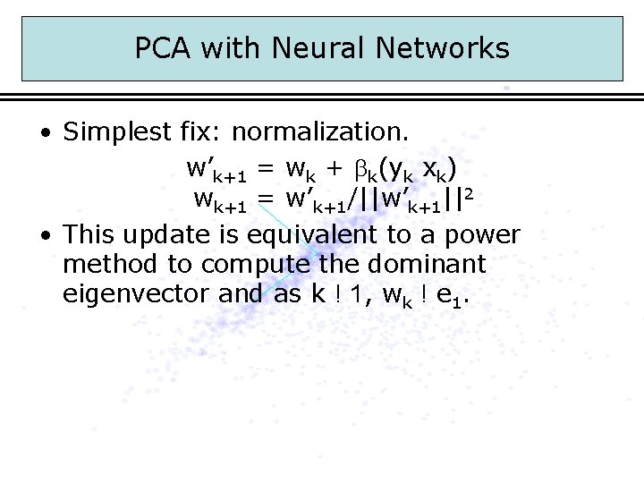
PCA with Neural Networks • Simplest fix: normalization. w’k+1 = wk + k(yk xk) wk+1 = w’k+1/||w’k+1||2 • This update is equivalent to a power method to compute the dominant eigenvector and as k ! 1, wk ! e 1.

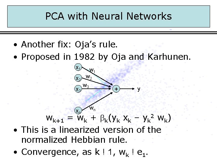
PCA with Neural Networks • Another fix: Oja’s rule. • Proposed in 1982 by Oja and Karhunen. x 1 x 2 x 3 xn w 1 w 2 w 3 + y wn wk+1 = wk + k(yk xk – yk 2 wk) • This is a linearized version of the normalized Hebbian rule. • Convergence, as k ! 1, wk ! e 1.

PCA with Neural Networks • Subspace Model • APEX • Multi-layer auto-associative.

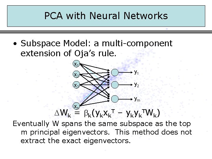
PCA with Neural Networks • Subspace Model: a multi-component extension of Oja’s rule. x 1 x 2 x 3 y 1 y 2 ym xn Wk = k(ykxk. T – ykyk. TWk) Eventually W spans the same subspace as the top m principal eigenvectors. This method does not extract the exact eigenvectors.

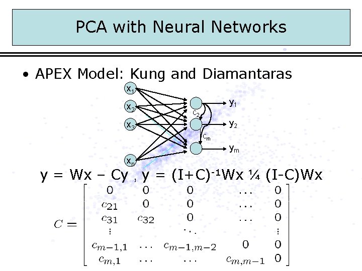
PCA with Neural Networks • APEX Model: Kung and Diamantaras x 1 x 2 x 3 y 1 c 2 y 2 cm ym xn y = Wx – Cy , y = (I+C)-1 Wx ¼ (I-C)Wx

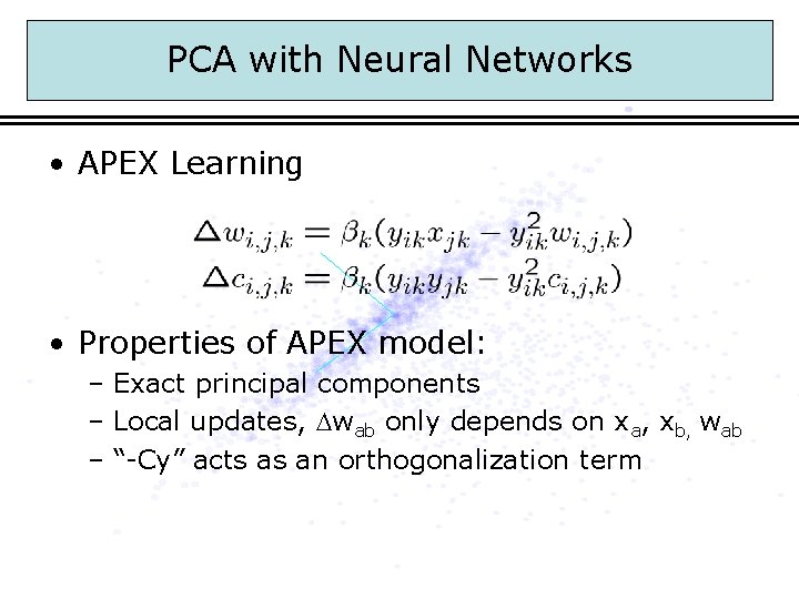
PCA with Neural Networks • APEX Learning • Properties of APEX model: – Exact principal components – Local updates, wab only depends on xa, xb, wab – “-Cy” acts as an orthogonalization term

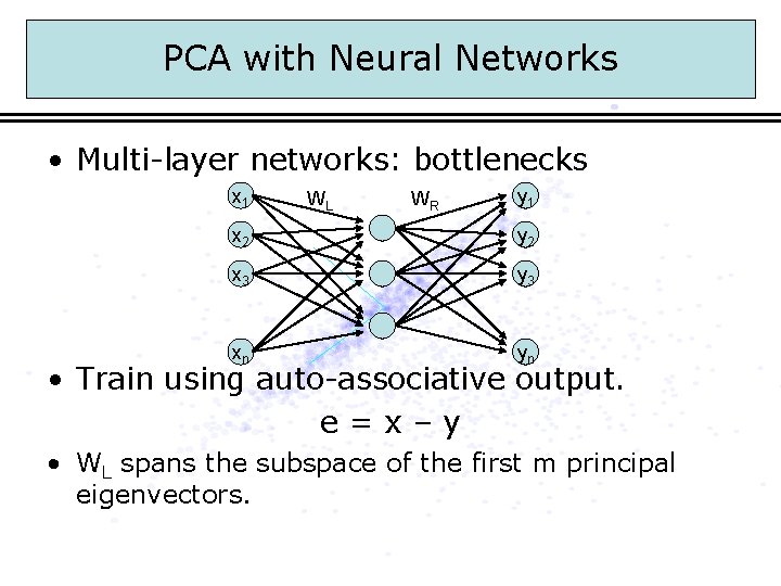
PCA with Neural Networks • Multi-layer networks: bottlenecks x 1 WL WR y 1 x 2 y 2 x 3 y 3 xn yn • Train using auto-associative output. e=x–y • WL spans the subspace of the first m principal eigenvectors.

Outline • Principal Component Analysis – Introduction – Linear Algebra Approach – Neural Network Implementation • Independent Component Analysis – Introduction – Demos – Neural Network Implementations • References • Questions

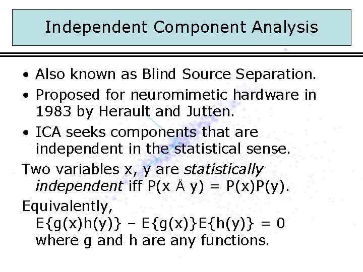
Independent Component Analysis • Also known as Blind Source Separation. • Proposed for neuromimetic hardware in 1983 by Herault and Jutten. • ICA seeks components that are independent in the statistical sense. Two variables x, y are statistically independent iff P(x Å y) = P(x)P(y). Equivalently, E{g(x)h(y)} – E{g(x)}E{h(y)} = 0 where g and h are any functions.

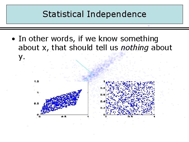
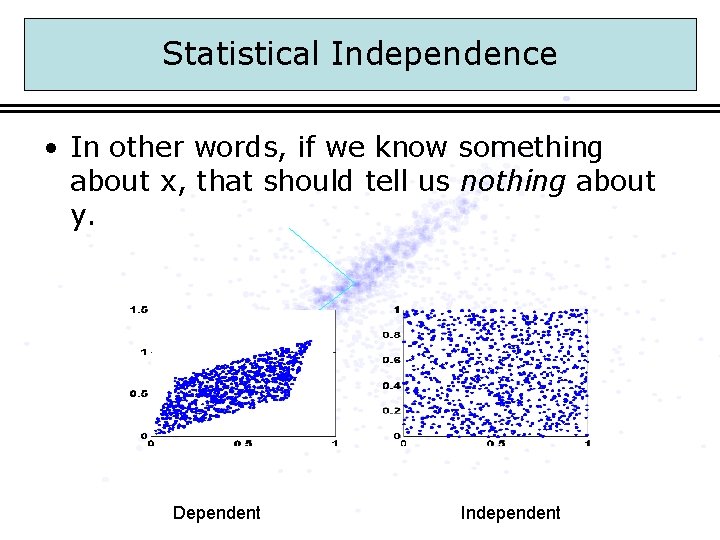
Statistical Independence • In other words, if we know something about x, that should tell us nothing about y.

Statistical Independence • In other words, if we know something about x, that should tell us nothing about y. Dependent Independent

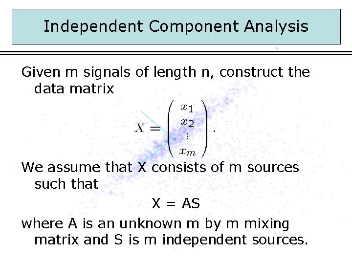
Independent Component Analysis Given m signals of length n, construct the data matrix We assume that X consists of m sources such that X = AS where A is an unknown m by m mixing matrix and S is m independent sources.

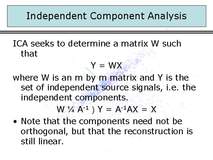
Independent Component Analysis ICA seeks to determine a matrix W such that Y = WX where W is an m by m matrix and Y is the set of independent source signals, i. e. the independent components. W ¼ A-1 ) Y = A-1 AX = X • Note that the components need not be orthogonal, but that the reconstruction is still linear.

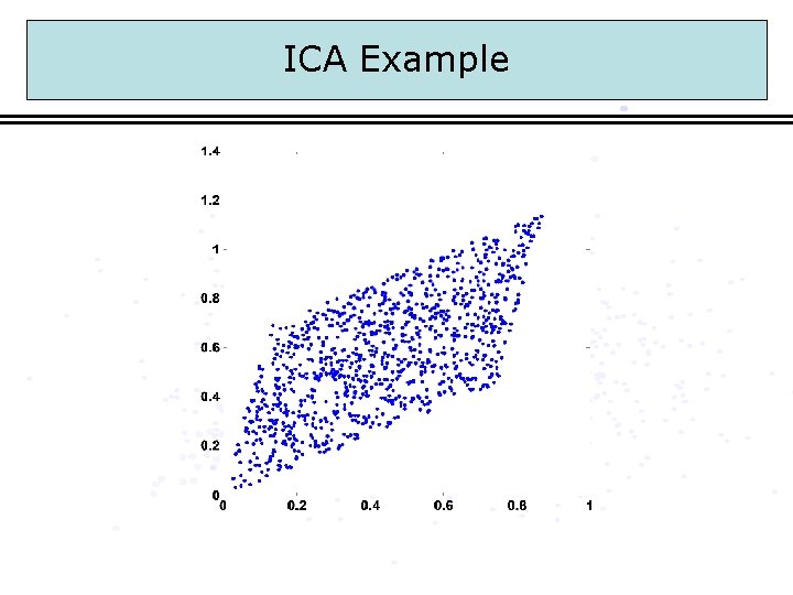
ICA Example

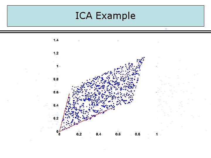
ICA Example

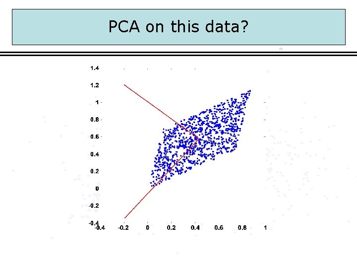
PCA on this data?

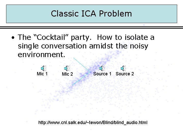
Classic ICA Problem • The “Cocktail” party. How to isolate a single conversation amidst the noisy environment. Mic 1 Mic 2 Source 1 Source 2 http: //www. cnl. salk. edu/~tewon/Blind/blind_audio. html

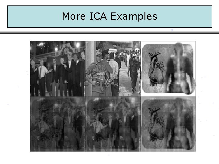
More ICA Examples

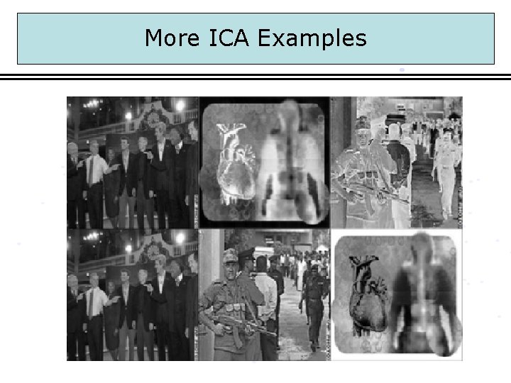
More ICA Examples

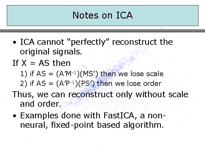
Notes on ICA • ICA cannot “perfectly” reconstruct the original signals. If X = AS then 1) if AS = (A’M-1)(MS’) then we lose scale 2) if AS = (A’P-1)(PS’) then we lose order Thus, we can reconstruct only without scale and order. • Examples done with Fast. ICA, a nonneural, fixed-point based algorithm.

Neural ICA • ICA is typically posed as an optimization problem. • Many iterative solutions to optimization problems can be cast into a neural network.

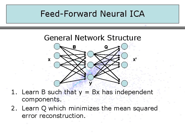
Feed-Forward Neural ICA General Network Structure B Q x x’ y 1. Learn B such that y = Bx has independent components. 2. Learn Q which minimizes the mean squared error reconstruction.

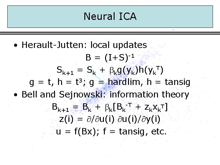
Neural ICA • Herault-Jutten: local updates B = (I+S)-1 Sk+1 = Sk + kg(yk)h(yk. T) g = t, h = t 3; g = hardlim, h = tansig • Bell and Sejnowski: information theory Bk+1 = Bk + k[Bk-T + zkxk. T] z(i) = / u(i)/ y(i) u = f(Bx); f = tansig, etc.

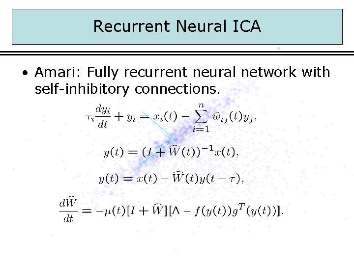
Recurrent Neural ICA • Amari: Fully recurrent neural network with self-inhibitory connections.

References • Diamantras, K. I. and S. Y. Kung. Principal Component Neural Networks. • Comon, P. “Independent Component Analysis, a new concept? ” In Signal Processing, vol. 36, pp. 287 -314, 1994. • Fast. ICA, http: //www. cis. hut. fi/projects/ica/fastica/ • Oursland, A. , J. D. Paula, and N. Mahmood. “Case Studies in Independent Component Analysis. ” • Weingessel, A. “An Analysis of Learning Algorithms in PCA and SVD Neural Networks. ” • Karhunen, J. “Neural Approaches to Independent Component Analysis. ” • Amari, S. , A. Cichocki, and H. H. Yang. “Recurrent Neural Networks for Blind Separation of Sources. ”

Questions?