Prims algorithm 1 Outline This topic covers Prims

Prim’s algorithm 1 Outline This topic covers Prim’s algorithm: – Finding a minimum spanning tree – The idea and the algorithm – An example

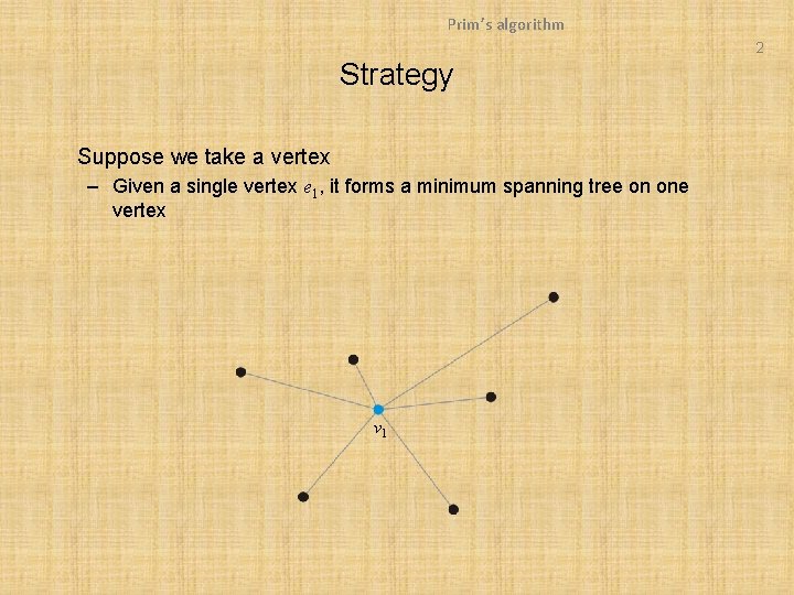
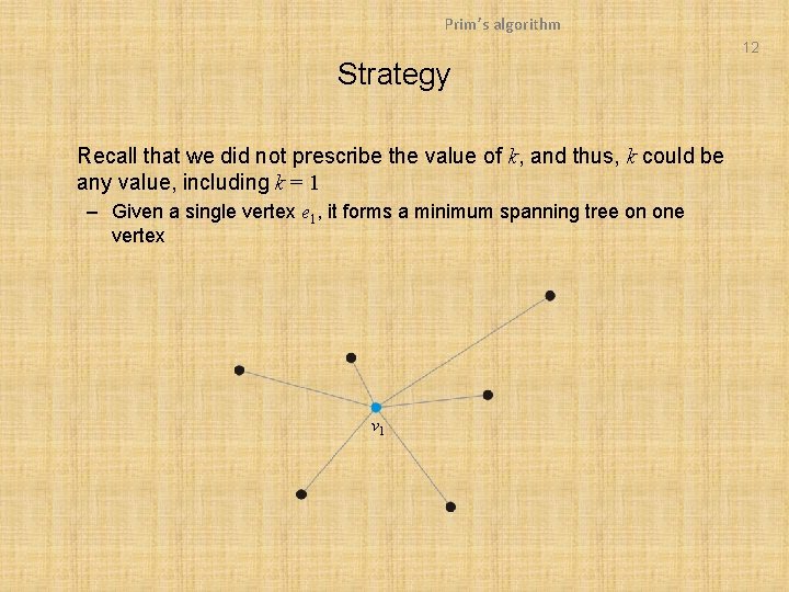
Prim’s algorithm 2 Strategy Suppose we take a vertex – Given a single vertex e 1, it forms a minimum spanning tree on one vertex v 1

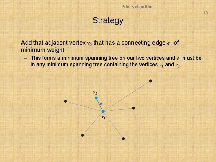
Prim’s algorithm 3 Strategy Add that adjacent vertex v 2 that has a connecting edge e 1 of minimum weight – This forms a minimum spanning tree on our two vertices and e 1 must be in any minimum spanning tree containing the vertices v 1 and v 2 e 1 v 1

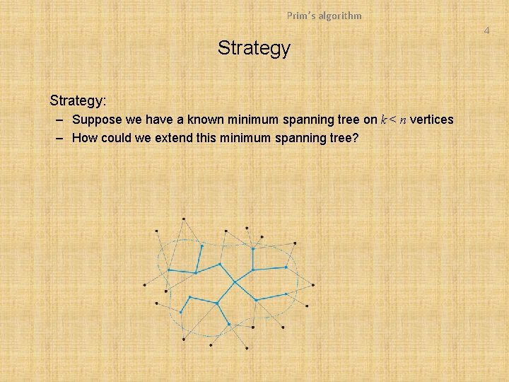
Prim’s algorithm 4 Strategy: – Suppose we have a known minimum spanning tree on k < n vertices – How could we extend this minimum spanning tree?

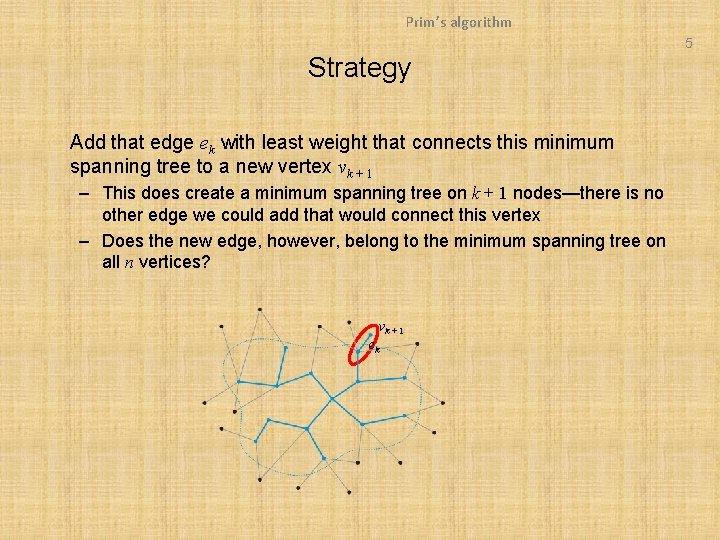
Prim’s algorithm 5 Strategy Add that edge ek with least weight that connects this minimum spanning tree to a new vertex vk + 1 – This does create a minimum spanning tree on k + 1 nodes—there is no other edge we could add that would connect this vertex – Does the new edge, however, belong to the minimum spanning tree on all n vertices? vk + 1 ek

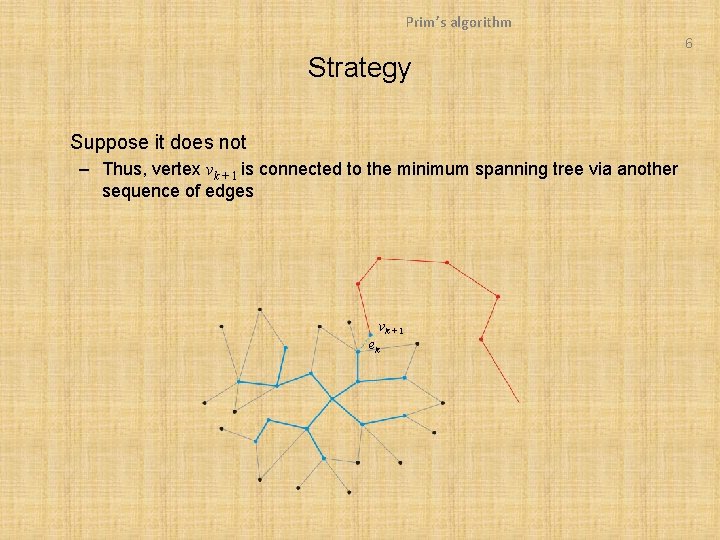
Prim’s algorithm 6 Strategy Suppose it does not – Thus, vertex vk + 1 is connected to the minimum spanning tree via another sequence of edges vk + 1 ek

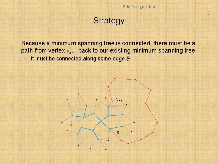
Prim’s algorithm 7 Strategy Because a minimum spanning tree is connected, there must be a path from vertex vk + 1 back to our existing minimum spanning tree – It must be connected along some edge vk + 1 ek

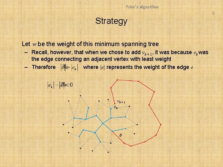
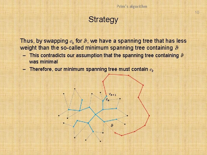
Prim’s algorithm 8 Strategy Let w be the weight of this minimum spanning tree – Recall, however, that when we chose to add vk + 1, it was because ek was the edge connecting an adjacent vertex with least weight – Therefore where |e| represents the weight of the edge e vk + 1 ek

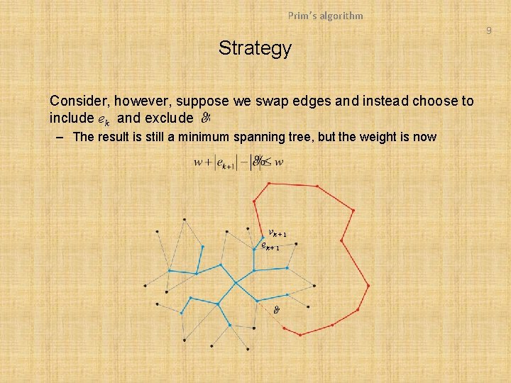
Prim’s algorithm 9 Strategy Consider, however, suppose we swap edges and instead choose to include ek and exclude – The result is still a minimum spanning tree, but the weight is now vk + 1 ek + 1

Prim’s algorithm 10 Strategy Thus, by swapping ek for , we have a spanning tree that has less weight than the so-called minimum spanning tree containing – This contradicts our assumption that the spanning tree containing was minimal – Therefore, our minimum spanning tree must contain ek vk + 1 ek

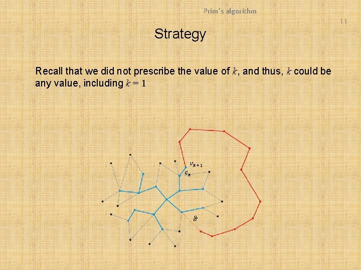
Prim’s algorithm 11 Strategy Recall that we did not prescribe the value of k, and thus, k could be any value, including k = 1 vk + 1 ek

Prim’s algorithm 12 Strategy Recall that we did not prescribe the value of k, and thus, k could be any value, including k = 1 – Given a single vertex e 1, it forms a minimum spanning tree on one vertex v 1

Prim’s algorithm 13 Strategy Add that adjacent vertex v 2 that has a connecting edge e 1 of minimum weight – This forms a minimum spanning tree on our two vertices and e 1 must be in any minimum spanning tree containing the vertices v 1 and v 2 e 1 v 1

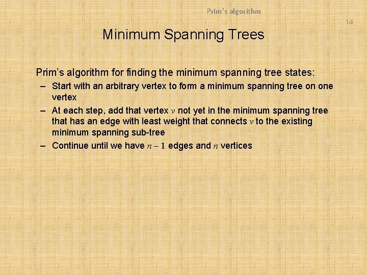
Prim’s algorithm 14 Minimum Spanning Trees Prim’s algorithm for finding the minimum spanning tree states: – Start with an arbitrary vertex to form a minimum spanning tree on one vertex – At each step, add that vertex v not yet in the minimum spanning tree that has an edge with least weight that connects v to the existing minimum spanning sub-tree – Continue until we have n – 1 edges and n vertices

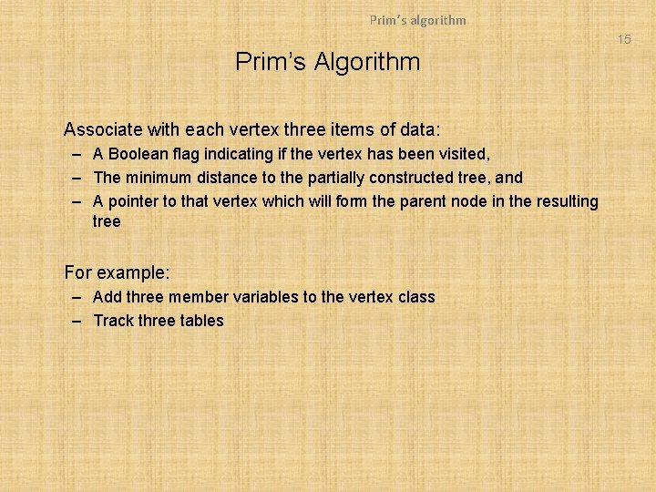
Prim’s algorithm 15 Prim’s Algorithm Associate with each vertex three items of data: – A Boolean flag indicating if the vertex has been visited, – The minimum distance to the partially constructed tree, and – A pointer to that vertex which will form the parent node in the resulting tree For example: – Add three member variables to the vertex class – Track three tables

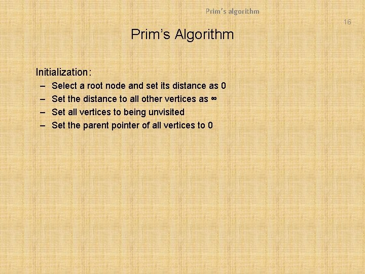
Prim’s algorithm 16 Prim’s Algorithm Initialization: – – Select a root node and set its distance as 0 Set the distance to all other vertices as ∞ Set all vertices to being unvisited Set the parent pointer of all vertices to 0

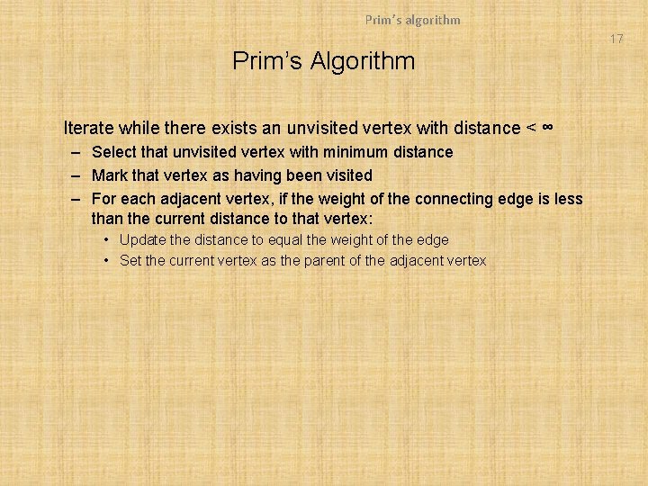
Prim’s algorithm 17 Prim’s Algorithm Iterate while there exists an unvisited vertex with distance < ∞ – Select that unvisited vertex with minimum distance – Mark that vertex as having been visited – For each adjacent vertex, if the weight of the connecting edge is less than the current distance to that vertex: • Update the distance to equal the weight of the edge • Set the current vertex as the parent of the adjacent vertex

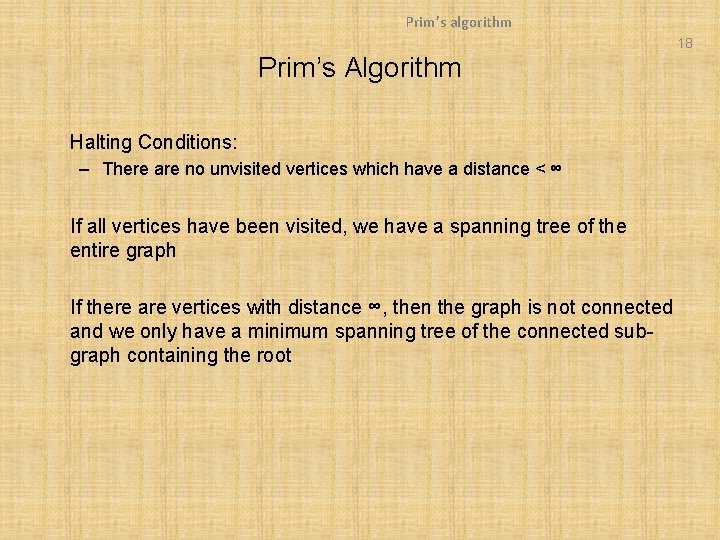
Prim’s algorithm 18 Prim’s Algorithm Halting Conditions: – There are no unvisited vertices which have a distance < ∞ If all vertices have been visited, we have a spanning tree of the entire graph If there are vertices with distance ∞, then the graph is not connected and we only have a minimum spanning tree of the connected subgraph containing the root

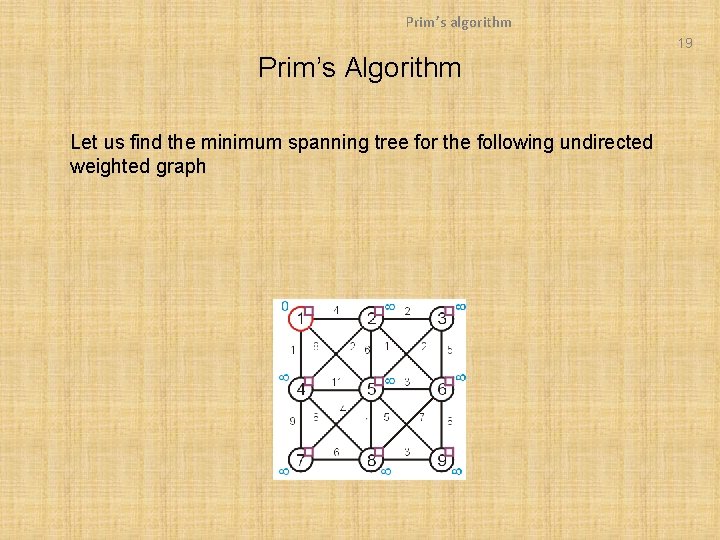
Prim’s algorithm 19 Prim’s Algorithm Let us find the minimum spanning tree for the following undirected weighted graph

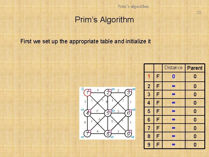
Prim’s algorithm 20 Prim’s Algorithm First we set up the appropriate table and initialize it Distance Parent 1 F 0 0 2 F ∞ 0 3 F ∞ 0 4 F ∞ 0 5 F ∞ 0 6 F ∞ 0 7 F ∞ 0 8 F ∞ 0 9 F ∞ 0

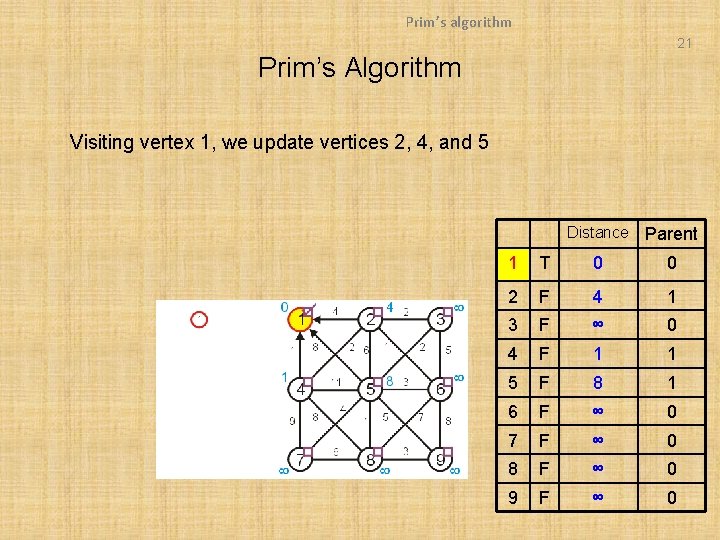
Prim’s algorithm 21 Prim’s Algorithm Visiting vertex 1, we update vertices 2, 4, and 5 Distance Parent 1 T 0 0 2 F 4 1 3 F ∞ 0 4 F 1 1 5 F 8 1 6 F ∞ 0 7 F ∞ 0 8 F ∞ 0 9 F ∞ 0

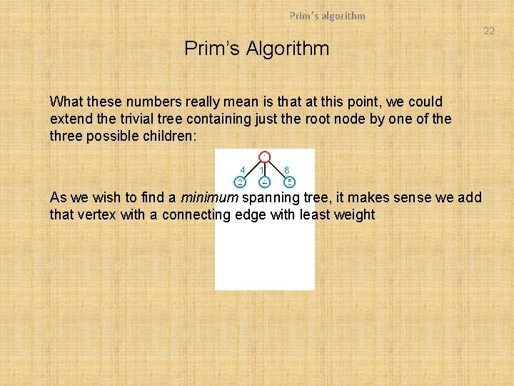
Prim’s algorithm 22 Prim’s Algorithm What these numbers really mean is that at this point, we could extend the trivial tree containing just the root node by one of the three possible children: As we wish to find a minimum spanning tree, it makes sense we add that vertex with a connecting edge with least weight

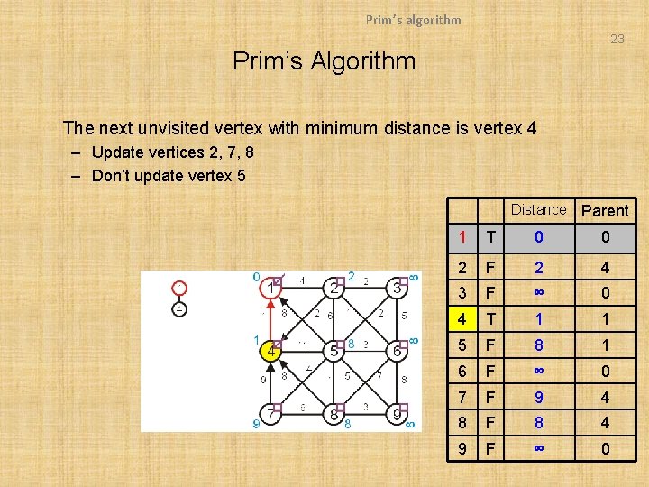
Prim’s algorithm 23 Prim’s Algorithm The next unvisited vertex with minimum distance is vertex 4 – Update vertices 2, 7, 8 – Don’t update vertex 5 Distance Parent 1 T 0 0 2 F 2 4 3 F ∞ 0 4 T 1 1 5 F 8 1 6 F ∞ 0 7 F 9 4 8 F 8 4 9 F ∞ 0

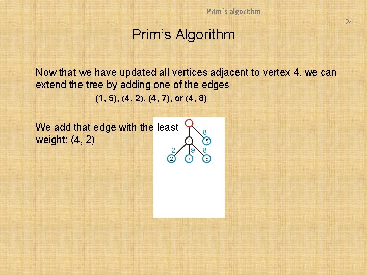
Prim’s algorithm 24 Prim’s Algorithm Now that we have updated all vertices adjacent to vertex 4, we can extend the tree by adding one of the edges (1, 5), (4, 2), (4, 7), or (4, 8) We add that edge with the least weight: (4, 2)

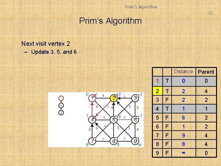
Prim’s algorithm 25 Prim’s Algorithm Next visit vertex 2 – Update 3, 5, and 6 Distance Parent 1 T 0 0 2 T 2 4 3 F 2 2 4 T 1 1 5 F 6 2 6 F 1 2 7 F 9 4 8 F 8 4 9 F ∞ 0

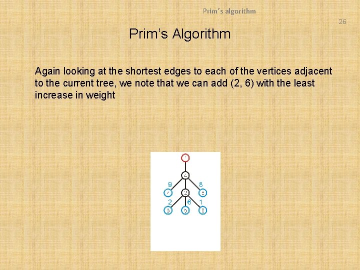
Prim’s algorithm 26 Prim’s Algorithm Again looking at the shortest edges to each of the vertices adjacent to the current tree, we note that we can add (2, 6) with the least increase in weight

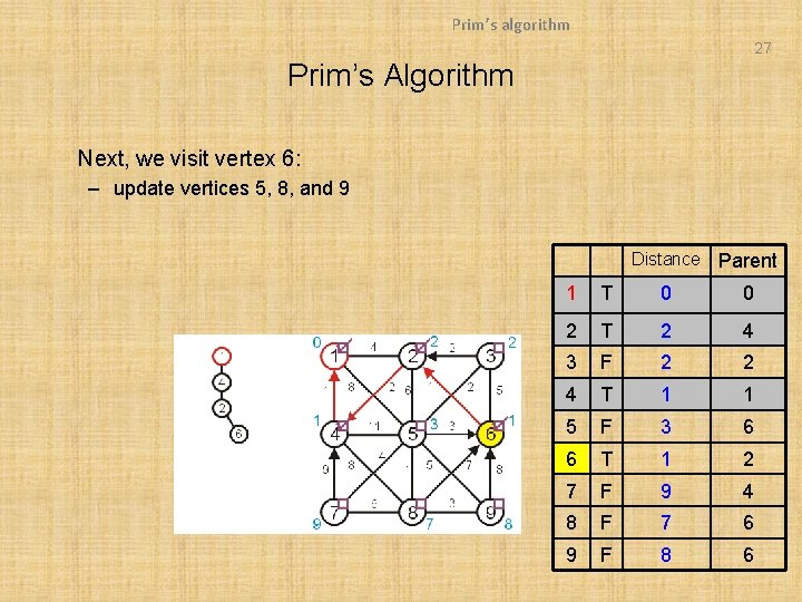
Prim’s algorithm 27 Prim’s Algorithm Next, we visit vertex 6: – update vertices 5, 8, and 9 Distance Parent 1 T 0 0 2 T 2 4 3 F 2 2 4 T 1 1 5 F 3 6 6 T 1 2 7 F 9 4 8 F 7 6 9 F 8 6

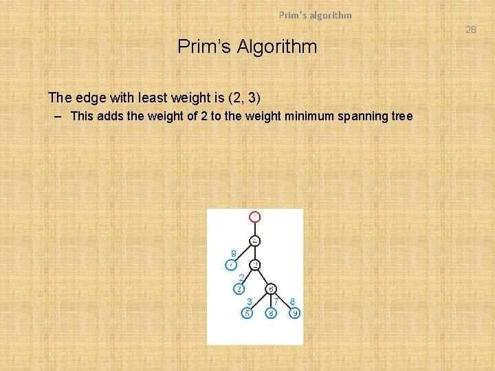
Prim’s algorithm 28 Prim’s Algorithm The edge with least weight is (2, 3) – This adds the weight of 2 to the weight minimum spanning tree

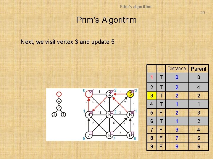
Prim’s algorithm 29 Prim’s Algorithm Next, we visit vertex 3 and update 5 Distance Parent 1 T 0 0 2 T 2 4 3 T 2 2 4 T 1 1 5 F 2 3 6 T 1 2 7 F 9 4 8 F 7 6 9 F 8 6

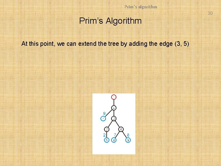
Prim’s algorithm 30 Prim’s Algorithm At this point, we can extend the tree by adding the edge (3, 5)

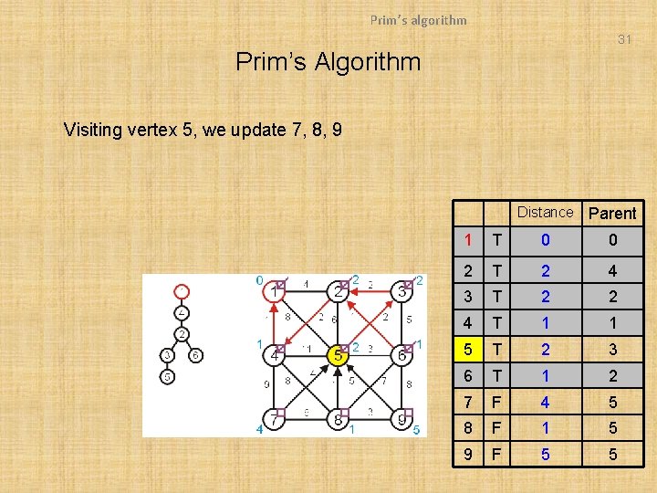
Prim’s algorithm 31 Prim’s Algorithm Visiting vertex 5, we update 7, 8, 9 Distance Parent 1 T 0 0 2 T 2 4 3 T 2 2 4 T 1 1 5 T 2 3 6 T 1 2 7 F 4 5 8 F 1 5 9 F 5 5

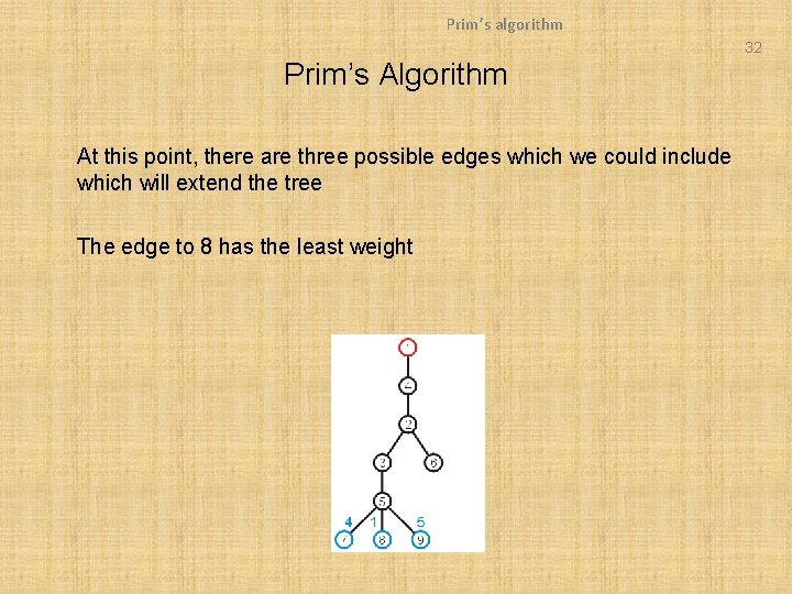
Prim’s algorithm 32 Prim’s Algorithm At this point, there are three possible edges which we could include which will extend the tree The edge to 8 has the least weight

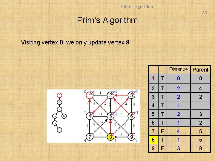
Prim’s algorithm 33 Prim’s Algorithm Visiting vertex 8, we only update vertex 9 Distance Parent 1 T 0 0 2 T 2 4 3 T 2 2 4 T 1 1 5 T 2 3 6 T 1 2 7 F 4 5 8 T 1 5 9 F 3 8

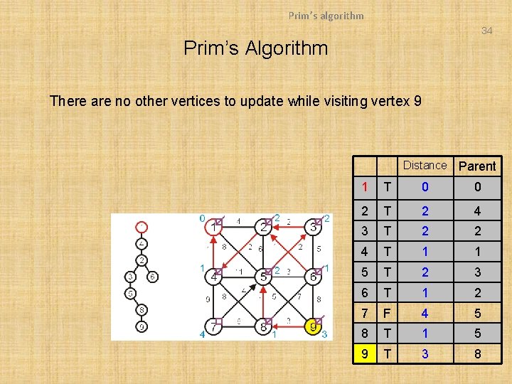
Prim’s algorithm 34 Prim’s Algorithm There are no other vertices to update while visiting vertex 9 Distance Parent 1 T 0 0 2 T 2 4 3 T 2 2 4 T 1 1 5 T 2 3 6 T 1 2 7 F 4 5 8 T 1 5 9 T 3 8

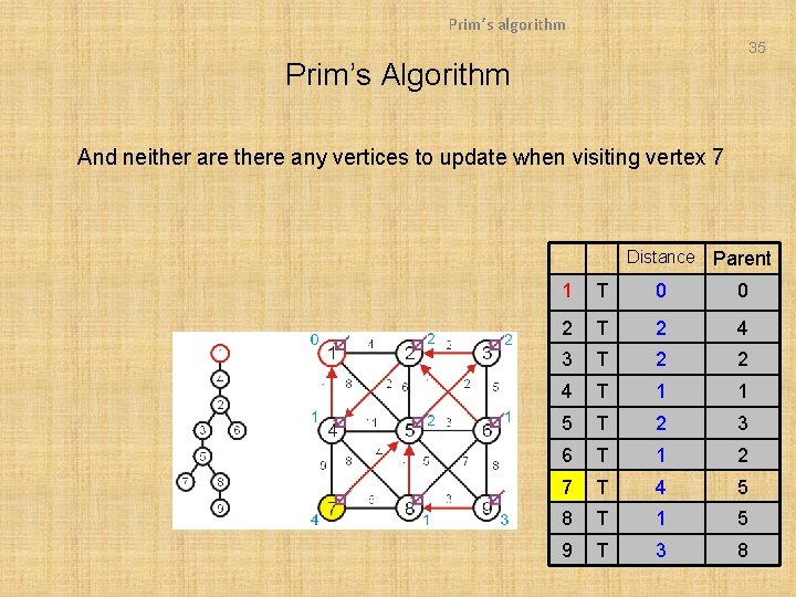
Prim’s algorithm 35 Prim’s Algorithm And neither are there any vertices to update when visiting vertex 7 Distance Parent 1 T 0 0 2 T 2 4 3 T 2 2 4 T 1 1 5 T 2 3 6 T 1 2 7 T 4 5 8 T 1 5 9 T 3 8

Prim’s algorithm 36 Prim’s Algorithm At this point, there are no more unvisited vertices, and therefore we are done If at any point, all remaining vertices had a distance of ∞, this would indicate that the graph is not connected – in this case, the minimum spanning tree would only span one connected sub-graph

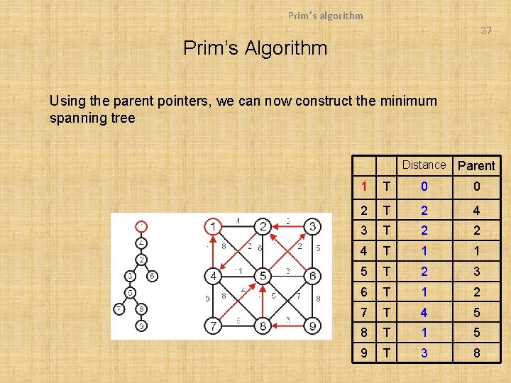
Prim’s algorithm 37 Prim’s Algorithm Using the parent pointers, we can now construct the minimum spanning tree Distance Parent 1 T 0 0 2 T 2 4 3 T 2 2 4 T 1 1 5 T 2 3 6 T 1 2 7 T 4 5 8 T 1 5 9 T 3 8

Prim’s algorithm 38 Prim’s Algorithm To summarize: – we begin with a vertex which represents the root – starting with this trivial tree and iteration, we find the shortest edge which we can add to this already existing tree to expand it This is a reasonably efficient algorithm: the number of visits to vertices is kept to a minimum

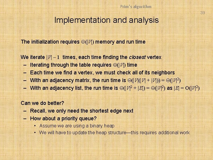
Prim’s algorithm 39 Implementation and analysis The initialization requires Q(|V|) memory and run time We iterate |V| – 1 times, each time finding the closest vertex – Iterating through the table requires Q(|V|) time – Each time we find a vertex, we must check all of its neighbors – With an adjacency matrix, the run time is Q(|V| + |V|)) = Q(|V|2) – With an adjacency list, the run time is Q(|V|2 + |E|) = Q(|V|2) as |E| = O(|V|2) Can we do better? – Recall, we only need the shortest edge next – How about a priority queue? • Assume we are using a binary heap • We will have to update the heap structure—this requires additional work

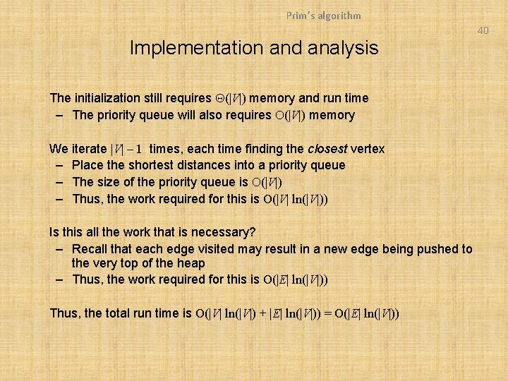
Prim’s algorithm 40 Implementation and analysis The initialization still requires Q(|V|) memory and run time – The priority queue will also requires O(|V|) memory We iterate |V| – 1 times, each time finding the closest vertex – Place the shortest distances into a priority queue – The size of the priority queue is O(|V|) – Thus, the work required for this is O(|V| ln(|V|)) Is this all the work that is necessary? – Recall that each edge visited may result in a new edge being pushed to the very top of the heap – Thus, the work required for this is O(|E| ln(|V|)) Thus, the total run time is O(|V| ln(|V|) + |E| ln(|V|)) = O(|E| ln(|V|))

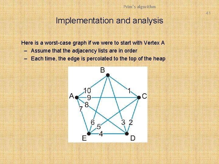
Prim’s algorithm 41 Implementation and analysis Here is a worst-case graph if we were to start with Vertex A – Assume that the adjacency lists are in order – Each time, the edge is percolated to the top of the heap

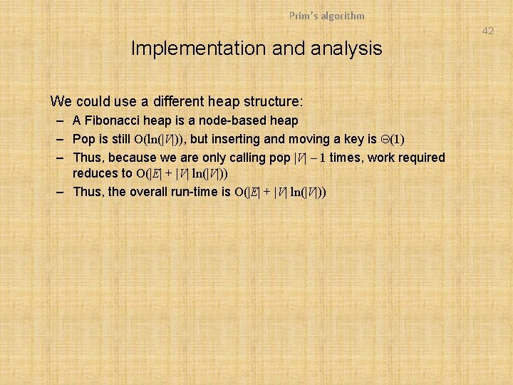
Prim’s algorithm 42 Implementation and analysis We could use a different heap structure: – A Fibonacci heap is a node-based heap – Pop is still O(ln(|V|)), but inserting and moving a key is Q(1) – Thus, because we are only calling pop |V| – 1 times, work required reduces to O(|E| + |V| ln(|V|)) – Thus, the overall run-time is O(|E| + |V| ln(|V|))

Prim’s algorithm 43 Implementation and analysis Thus, we have two run times when using – A binary heap: O(|E| ln(|V|)) – A Fibonacci heap: O(|E| + |V| ln(|V|)) Questions: Which is faster if |E| = Q(|V|)? How about if |E| = Q(|V|2)?

Prim’s algorithm 44 Summary We have seen an algorithm for finding minimum spanning trees – Start with a trivial minimum spanning tree and grow it – An alternate algorithm, Kruskal’s algorithm, uses a different approach Prim’s algorithm finds an edge with least weight which grows an already existing tree – It solves the problem in O(|E| ln(|V|)) time

Prim’s algorithm 45 References Wikipedia, http: //en. wikipedia. org/wiki/Minimum_spanning_tree Wikipedia, http: //en. wikipedia. org/wiki/Prim’s_algorithm These slides are provided for the ECE 250 Algorithms and Data Structures course. The material in it reflects Douglas W. Harder’s best judgment in light of the information available to him at the time of preparation. Any reliance on these course slides by any party for any other purpose are the responsibility of such parties. Douglas W. Harder accepts no responsibility for damages, if any, suffered by any party as a result of decisions made or actions based on these course slides for any other purpose than that for which it was intended.