Price Discrimination Upper 6 th Micro Pricing Strategies

Price Discrimination Upper 6 th Micro Pricing Strategies

Intro to Price Discrimination Mr O’Grady

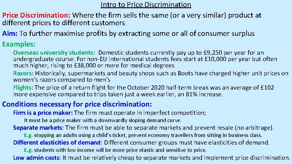
Intro to Price Discrimination: Where the firm sells the same (or a very similar) product at different prices to different customers Aim: To further maximise profits by extracting some or all of consumer surplus Examples: Overseas university students: Domestic students currently pay up to £ 9, 250 per year for an undergraduate course. For non-EU international students fees start at £ 10, 000 per year but often much higher, rising to £ 38, 000 or more for medical degrees Razors: Historically, supermarkets and beauty shops such as Boots have charged higher unit prices on women’s razors compared to men’s Flights: The price of a return flight for the October 2020 half-term break was an average of £ 102 more expensive compared to trips taken just a week earlier, an 81% increase. Conditions necessary for price discrimination: Firm is a price maker: The firm must operate in imperfect competition; It must be a price maker with a downwardly sloping demand curve. Separate markets: The firm must be able to separate markets and prevent resale (no arbitrage). E. g. stopping an adults using a child’s ticket, prevent economy travellers from sitting in business class. Different elasticities of demand: Different consumer groups must have elasticities of demand. E. g. students with low income will be more price elastic and sensitive to price. Low admin costs: It must be relatively cheap to separate markets and implement price discrimination.

First Degree Price Discrimination Mr O’Grady

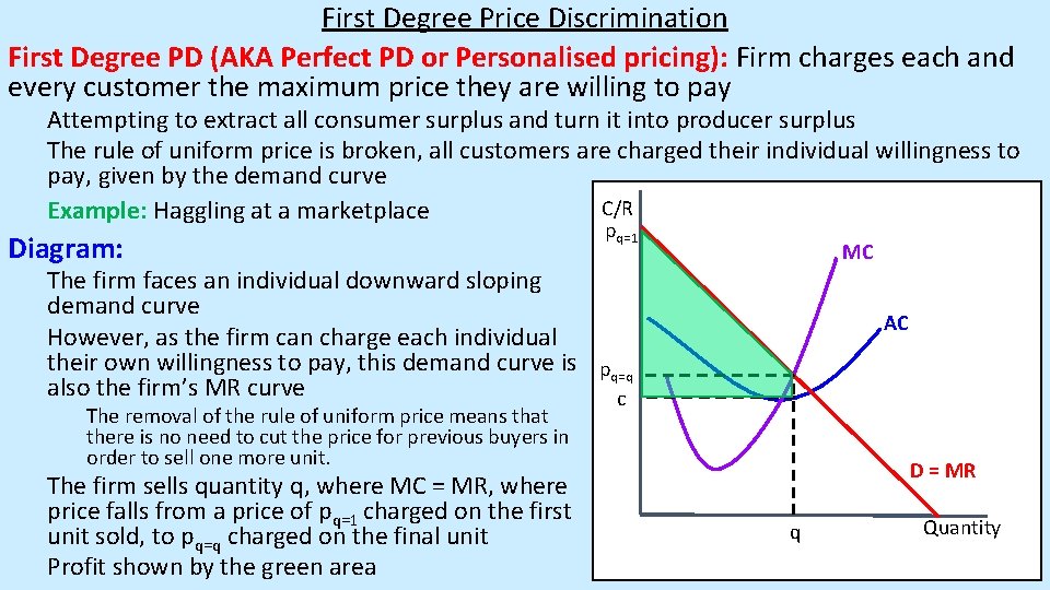
First Degree Price Discrimination First Degree PD (AKA Perfect PD or Personalised pricing): Firm charges each and every customer the maximum price they are willing to pay Attempting to extract all consumer surplus and turn it into producer surplus The rule of uniform price is broken, all customers are charged their individual willingness to pay, given by the demand curve C/R Example: Haggling at a marketplace Diagram: pq=1 MC The firm faces an individual downward sloping demand curve However, as the firm can charge each individual their own willingness to pay, this demand curve is pq=q also the firm’s MR curve c AC The removal of the rule of uniform price means that there is no need to cut the price for previous buyers in order to sell one more unit. The firm sells quantity q, where MC = MR, where price falls from a price of pq=1 charged on the first unit sold, to pq=q charged on the final unit Profit shown by the green area D = MR q Quantity

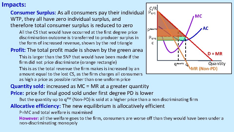
Impacts: Consumer Surplus: As all consumers pay their individual WTP, they all have zero individual surplus, and therefore total consumer surplus is reduced to zero All the CS that would have occurred at the first degree price discrimination outcome is transferred to producer surplus in the form of increased revenue, shown by the red triangle C/R pq=1 MC AC p. Non-PD pq=q c Profit: The total profit made is shown by the green area This is larger than the SNP that would have been made if the firm did not price discriminate (orange rectangle) This is as the total revenue the firm makes is increased by an amount equal to the lost CS, as the firm charges all consumers as high a price as possible rather than one uniform price D = MR q. Non-PD q Quantity MR (Non-PD) Quantity sold: increased as MC = MR at a greater quantity Price: price for final good sold under first degree PD is lower But the quantity up to q. PM (Non-PD) is sold at a higher price than a non discriminating firm Allocative efficiency: The new equilibrium is allocatively efficient P=MC and total welfare is maximised However: all the welfare goes to the firm, consumers are worse off than they would have been under a non-discriminating monopoly

Second Degree Price Discrimination Mr O’Grady

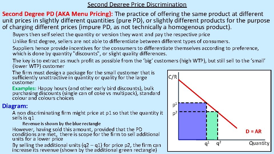
Second Degree Price Discrimination Second Degree PD (AKA Menu Pricing): The practice of offering the same product at different unit prices in slightly different quantities (pure PD), or slightly different products for the purpose of charging different prices (impure PD, as not technically a homogenous product). Buyers then self select the quantity or version they want and pay the respective price Unlike first degree, sellers are not able to differentiate between different types of consumers. Suppliers hence provide incentives for the consumers to differentiate themselves according to preference, which is done by quantity "discounts", or slight quality differences. The key is to extract as much profit as possible from the ‘big’ customers (high WTP), but still sell to the ‘small’ (lower WTP) customer The firm must design a package for the small customer that is C/R sufficiently unattractive in quantity or quality for the large customer Examples: Happy hours (and other early bird discounts), bulk purchasing discounts (single can of coke vs multipack), standard colour and colours choices p 1 Diagram: A non discriminating firm might price at p 1 so that the quantity it p 2 sells is q 1 Revenue is shown by the blue rectangle However, having sold this amount, provided that the PD conditions are met, there is scope for the firm to sell additional units for a lower price By selling the additional units (q 2 – q 1) for price p 2, the firm can increase its revenue (shown by the additional green rectangle) D = AR q 1 q 2 Quantity

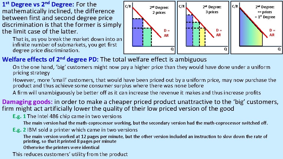
1 st Degree vs 2 nd Degree: For the mathematically inclined, the difference between first and second degree price discrimination is that the former is simply the limit case of the latter. C/R That is, as you break the market down into an infinite number of submarkets, you get first degree price discrimination. C/R 2 nd Degree: 2 prices C/R 2 nd Degree: 3 prices 2 nd Degree: ∞ prices = 1 st Degree D= AR Q Q Welfare effects of 2 nd degree PD: The total welfare effect is ambiguous On the one hand, ‘big’ customers might now pay a higher price than they would have done under a uniform pricing strategy However, more ‘small’ customers, that would have been priced out by a uniform price, may now purchase the product and thus achieve some consumer surplus where there was none before A firm will unambiguously be better off as it can increase the revenue it makes and thus increase profits Damaging goods: in order to make a cheaper priced product unattractive to the ‘big’ customers, firm might act artificially lower the quality of their low priced version of the good E. g. 1 The Intel 486 chip came in two versions The main version had the math-coprocessor working, but the secondary version had the math-coprocessor switched off. E. g. 2 IBM sold a printer which came in two versions The main version worked at 12 pages per minute, but the other version included an instruction to slow down the rate of printing, so that it printed 8 pages per minute Otherwise the printers were identical This reduces customers’ utility from the product

Third Degree Price Discrimination Mr O’Grady

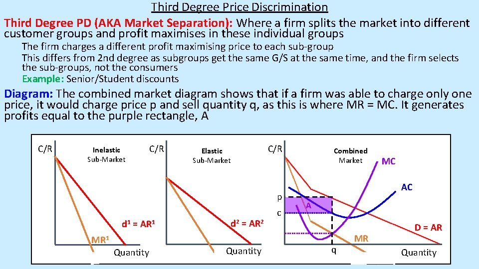
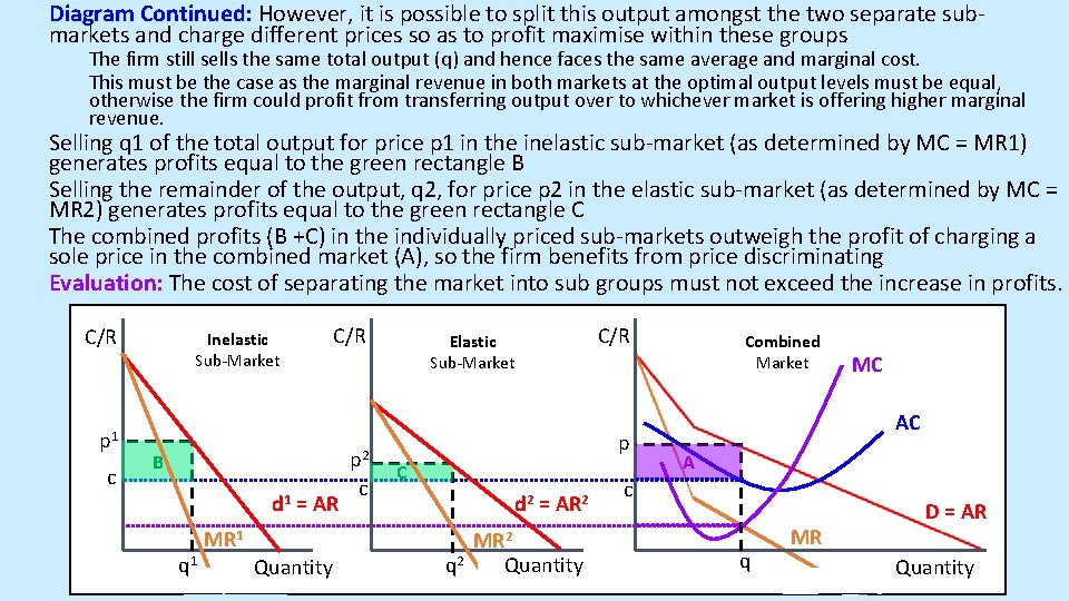
Third Degree Price Discrimination Third Degree PD (AKA Market Separation): Where a firm splits the market into different customer groups and profit maximises in these individual groups The firm charges a different profit maximising price to each sub-group This differs from 2 nd degree as subgroups get the same G/S at the same time, and the firm selects the sub-groups, not the consumers Example: Senior/Student discounts Diagram: The combined market diagram shows that if a firm was able to charge only one price, it would charge price p and sell quantity q, as this is where MR = MC. It generates profits equal to the purple rectangle, A C/R Inelastic Sub-Market C/R Elastic Sub-Market C/R p d 1 = AR 1 MR 1 Quantity d 2 = AR 2 Quantity c Combined Market MC AC A q MR D = AR Quantity

Diagram Continued: However, it is possible to split this output amongst the two separate submarkets and charge different prices so as to profit maximise within these groups The firm still sells the same total output (q) and hence faces the same average and marginal cost. This must be the case as the marginal revenue in both markets at the optimal output levels must be equal, otherwise the firm could profit from transferring output over to whichever market is offering higher marginal revenue. Selling q 1 of the total output for price p 1 in the inelastic sub-market (as determined by MC = MR 1) generates profits equal to the green rectangle B Selling the remainder of the output, q 2, for price p 2 in the elastic sub-market (as determined by MC = MR 2) generates profits equal to the green rectangle C The combined profits (B +C) in the individually priced sub-markets outweigh the profit of charging a sole price in the combined market (A), so the firm benefits from price discriminating Evaluation: The cost of separating the market into sub groups must not exceed the increase in profits. C/R p 1 c Inelastic Sub-Market C/R B d 1 = AR q 1 MR 1 Quantity p 2 c Elastic Sub-Market C/R p C d 2 = AR 2 MR 2 q 2 Quantity Combined Market MC AC A c q MR D = AR Quantity

Negative Impacts: Consumer surplus is reduced in most cases - representing a loss of welfare. For the majority of buyers, the price charged is well above the marginal cost of supply In increasing profits through price discrimination, consumer surplus is reduced and turned into producer surplus/profits Consumers are exploited and forced to pay higher prices well above MC for most Anticompetitive: Price discrimination also might be used as a predatory pricing tactic to harm competition and increase a firm's market power in the long run It can be illegal in some cases, and might be investigated by the CMA Positive Impacts: However: some consumers who can now buy the product at a lower price may benefit. Lower-income consumers may be "priced into the market" if the supplier is willing and able to charge them less. E. g. bursaries for universities Profits made in one market may allow firms to cross-subsidise loss-making activities/services that have important social benefits. E. g. money made on commuter rail or bus services may allow transport companies to support loss-making rural or night time services. Dynamic efficiency: Higher SNP can encourage R&D and innovation lowering costs for all consumers in the future

Where next? Don’t forget to SUBSCRIBE! Visit our website: www. smootheconomics. co. uk Find more resources, extension materials, details of courses, competitions, and more! Follow our socials: Instagram: @smootheconomics Twitter: @Smooth. Economics Facebook: @Smooth. Economics