Pressure and Friction Drag II Boundary layers Hydromechanics

Pressure and Friction Drag II + Boundary layers Hydromechanics VVRN 35 ppt by Magnus Larson; revised by Rolf L Jan 2014, Jan 2018, Jan 2019, EN 2020

SYNOPSIS 1. 2. 3. 4. 5. 6. 7. 8. Drag – General Observations Drag Coefficients for Different Shapes Drag Coefficient for sphere in Laminar Flow / Stokes Law Vortex Shedding Examples/Problems Lift Force on Bodies Magnus Effect Boundary layers

Drag equation • Area? • For symmetrical shapes = Projected area facing the flow

Drag – General Observations Pressure drag depends on the pressure distribution around the body and therefore on the size of the separation zone. Large zone of separation Small zone of separation large drag force small drag force The location of separation points are decisive for the magnitude of the pressure drag. Such locations are determined by: • body shape • body roughness • flow conditions

Flow around Golf Ball I) Smooth surface Laminar boundary layer II) Surface with ”dimples” creates Turbulent boundary layer, which has stronger mixing ”Stronger” boundary layer Separation pt moves downstream => Smaller zone of separation and resulting drag force

Drag – General Observations 1. Dp >> Df 2. Dp Df 3. Dp << Df

Laminar and Turbulent Boundary Layers Ideal fluid symmetric flow Laminar conditions flow separation Turbulent conditions – separation point shifts position downstream

Stagnation • • Acceleration Decreasing pressure Friction Boundary layer stable • • Deceleration Increasing pressure Friction Boundary layer grows, decelerate, and reverses

Flow around Sphere Flow separation point Trip wire Flow separation point with trip wire

3. Drag Coefficients for Different Shapes Drag coefficient depends on Re and geometry (sphere, disk, streamlined body). Transition to turbulent boundary layer Cd Re = Vdρ/ μ Laminar flow Little variation with Re No separation

4. Drag Coefficient for sphere in Laminar Flow / Stokes Law Stokes derived the drag force for laminar conditions (viscous forces dominate): (eq. 1) General formulation of Drag force: (eq. 2) Equivalence [ eq. 1 and 2] yields: (eq. 3) George Stokes

With cross-sectional area: Cd (eq. 4) (eq. 3) Combine eq. 3 and eq. 4 and Solve for drag coefficient: Re = Vdρ/ μ Stokes equation valid for Re < 1

Example IV: Particle Sedimentation FB FD Sediment particle in water – what is the terminal speed? Newton-Stokes law of sedimentation (laminar flow) FG Stokes equation valid for Re < 1 Examples of settling tanks

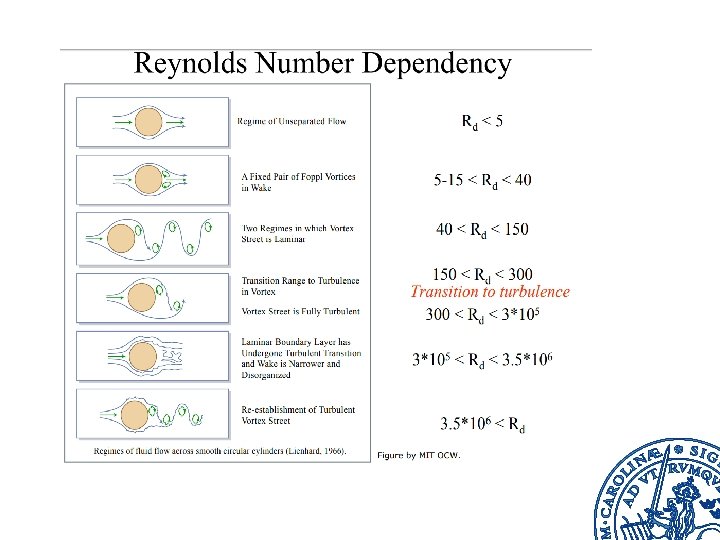
5. Vortex Shedding Under certain conditions vortices are generated from the edges of a body in a flow. Von Karman’s vortex street Theodore Von Karman Vortex street behind a cylinder

Vortices at Aleutian Islands (photo from space)

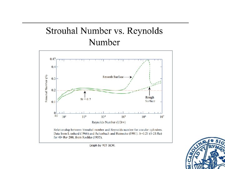
Regular vortex shedding may occur at a frequency n determined by Strouhal’s number: where n = frequency of vortex shedding d = typical length (diameter) V 0 = velocity (S = 0. 21 over a wide range of Re) Vincent Strouhal Periodic vortex shedding may lead to transversal forces on structures (e. g. , pipes, chimneys, bridges) resulting in vibration and possible structural damages. If it is close to the natural frequency of the structure, large effects are expected.

6. Examples / problems Example I : Vortex Shedding from Antenna Stand What is the frequency of the vortices shed? 30 m wind 35 m/s 0. 3 m Standard atmosphere (101 k. Pa, 20 deg)

Case: Tacoma Bridge (US) Built 1940 Span: 2, 800 ft (850 m) Plate-girder deck: 8 ft (2. 4 m) Wind-induced vibrations caused oscillations of the deck with eventual collapse

Boundary Layers Hydromechanics VVR 090 ppt by Magnus L; revised by Rolf L Jan 2014, Feb 2015, Feb 2017, Feb 2019

SYNOPSIS 1. 2. 3. 4. 5. Boundar Layer on a Flat Plate Von Karman momentum integral equation Laminar Boundary Layer along a Flat Plate Drag Coefficient for Smooth, Flat Plates Examples/Problems Figure numbers and Equation numbers refer to Vennard and Street : Elementary Fluid Mechanics

1. Boundar Layer (BL) on a Flat Plate V 0 = free stream velocity (m/s) δ = boundary layer thickness (m) Fig. 13. 6 Boundary layer: the zone in which the velocity profile is governed by frictional action

Boundary layer characterized by two Reynold’s numbers: V 0 = free stream velocity (m/s) δ = boundary layer thickness (m) Different R Different ranges for flow regimes (in boundary layer): (Uo = V 0)

Laminar and turbulent boundary layers • Laminar boundary layer = flow is in layers • Small Re • Exchange of mass and momentum only between adjacent layers • Viscosity can predict shear stress • Turbulent boundary layer = mixing of layers • Large Re • Exchange of mass and momentum across layers

Laminar and turbulent boundary layers Height from object surface Different velocity profiles • Affects shear stress & heat transfer Velocity along object

Von Karman momentum integral equation • Apply momentum equation for control volume ABCD. • Height of control volume extends beyond the edge of the boundary layer (to the outer flow). • At edge of the boundary layer: po(x), Vo(x) (known). • Small curvature along body.

Von Karman momentum integral equation Velocity derivates of boundary layer: • Apply momentum equation for control volume ABCD. • Height of control volume extends beyond the edge of the boundary layer (to the outer flow). • At edge of the boundary layer: po(x), Vo(x) (known). • Small curvature along body.

Von Karman momentum integral equation Assume unit depth No flow through A-D mass flow rate through B-C: Mass flow rate through A-B Mass flow rate through C-D

Von Karman momentum integral equation Forces & momentum Mass flow rate through B-C Momentum flux out of control volume through A-B Momentum flux out through C-D Net momentum out of control volume:

Von Karman momentum integral equation Forces & momentum Forces on A-B & C-D Force on B-C With small height difference dδ over control volume Net force on control volume depends on pressure difference in s-direction and shear stress:

Von Karman momentum integral equation Euler equation for outer flow gives that pressure difference drives velocity difference: Momentum addition from changed flow rate Momentum difference Pressure difference in s-direction Shear stress

Von Karman momentum integral equation When applying momentum equation to laminar flow (parabolic velocity profile), can show that: V&S eq. 13. 15 (p 619) When applying momentum equation to turbulent flow (nonparabolic velocity profile), can show that: V&S eq. 13. 22 (p 622)

5. Examples / problems Example I: Boundary layer and drag on ship model A ship model 1. 5 m long and with a draft of 0. 15 m is towed at a velocity of 0. 3 m/s in a basin containing water at 16 C. Assuming that one side of the immersed portion of the hull may be approximated by a smooth flat plate (1. 5 m x 0, 15 m), estimate the frictional drag of the hull and the thickness of the boundary layer at the stern of the model if the boundary layer is a) laminar and b) turbulent.

5. Examples / problems Example I: Boundary layer and drag on ship model A ship model 1. 5 m long and with a draft of 0. 15 m is towed at a velocity of 0. 3 m/s in a basin containing water at 16 C. Assuming that one side of the immersed portion of the hull may be approximated by a smooth flat plate (1. 5 m x 0, 15 m), estimate the frictional drag of the hull and the thickness of the boundary layer at the stern of the model if the boundary layer is a) laminar

5. Examples / problems Example I: Boundary layer and drag on ship model A ship model 1. 5 m long and with a draft of 0. 15 m is towed at a velocity of 0. 3 m/s in a basin containing water at 16 C. Assuming that one side of the immersed portion of the hull may be approximated by a smooth flat plate (1. 5 m x 0, 15 m), estimate the frictional drag of the hull and the thickness of the boundary layer at the stern of the model if the boundary layer is a) laminar V&S eq. 13. 15 (p 619)

5. Examples / problems Example I: Boundary layer and drag on ship model A ship model 1. 5 m long and with a draft of 0. 15 m is towed at a velocity of 0. 3 m/s in a basin containing water at 16 C. Assuming that one side of the immersed portion of the hull may be approximated by a smooth flat plate (1. 5 m x 0, 15 m), estimate the frictional drag of the hull and the thickness of the boundary layer at the stern of the model if the boundary layer is b) turbulent V&S eq. 13. 22 (p 622)