Presentation Autocorrelation Introduction to Autocorrelation The error terms

Presentation: Autocorrelation

Introduction to Autocorrelation The error terms are correlated with one another. This violation of the classical econometric model is generally known as autocorrelation of the errors

Nature of Autocorrelation • Autocorrelation is a systematic pattern in the errors that can be either attracting (positive) or repelling (negative) autocorrelation. • Error occurring at period t may be carried over to the next period t+1. • Autocorrelation is most likely to occur in time series data. • For efficiency (accurate estimation/prediction) all systematic information needs to be incorporated into the regression model.

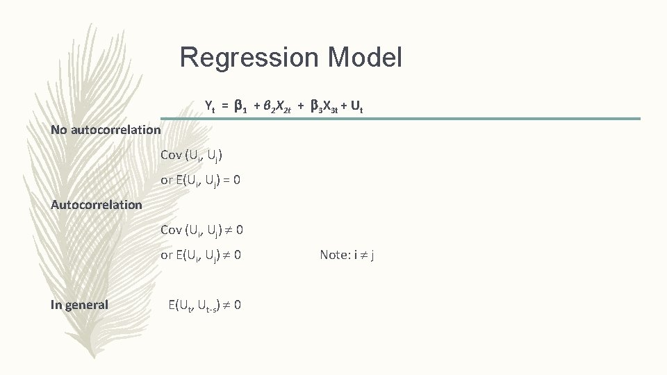
Regression Model Yt = 1 + β 2 X 2 t + 3 X 3 t + Ut No autocorrelation Cov (Ui, Uj) or E(Ui, Uj) = 0 Autocorrelation Cov (Ui, Uj) 0 or E(Ui, Uj) 0 In general E(Ut, Ut-s) 0 Note: i j

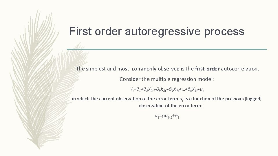
First order autoregressive process The simplest and most commonly observed is the first-order autocorrelation. Consider the multiple regression model: Yt=β 1+β 2 X 2 t+β 3 X 3 t+β 4 X 4 t+…+βk. Xkt+ut in which the current observation of the error term ut is a function of the previous (lagged) observation of the error term: ut=ρut-1+et

Continue…. The coefficient ρ is called the first-order autocorrelation coefficient and takes values form -1 to +1. It is obvious that the size of ρ will determine the strength of serial correlation.

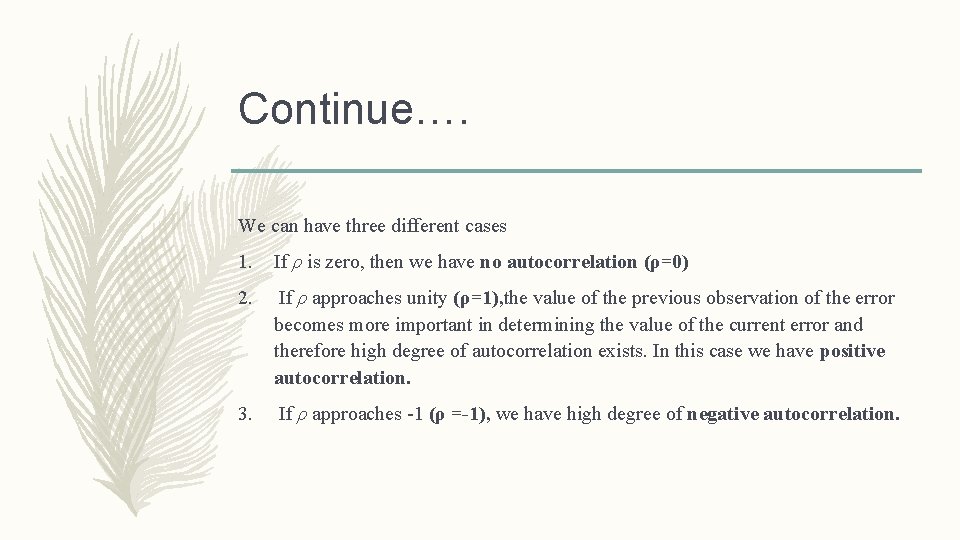
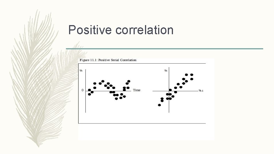
Continue…. We can have three different cases 1. If ρ is zero, then we have no autocorrelation (ρ=0) 2. If ρ approaches unity (ρ=1), the value of the previous observation of the error becomes more important in determining the value of the current error and therefore high degree of autocorrelation exists. In this case we have positive autocorrelation. 3. If ρ approaches -1 (ρ =-1), we have high degree of negative autocorrelation.

Positive correlation

Negative Correlation

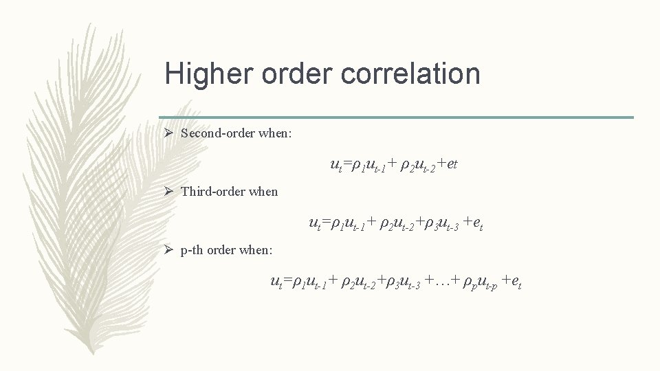
Higher order correlation Ø Second-order when: ut=ρ1 ut-1+ ρ2 ut-2+et Ø Third-order when ut=ρ1 ut-1+ ρ2 ut-2+ρ3 ut-3 +et Ø p-th order when: ut=ρ1 ut-1+ ρ2 ut-2+ρ3 ut-3 +…+ ρput-p +et

Causes of Autocorrelation is a common problem in time series regression. Several causes which give rise to autocorrelation as: • Omitted explanatory variables. • Misspecification of the mathematical form of the model. • Interpolation in the statistical observation. • Misspecification of the true error u.

Consequences of Autocorrelation 1. In the presence of autocorrelation the OLS estimators are still linear unbiased as well as consistent. 2. The OLS estimators will be inefficient and therefore no longer BLUE. 3. The estimated variances of the regression coefficients will be biased and inconsistent, and therefore hypothesis testing is no longer valid. In most of the cases, the R 2 will be overestimated and the t-statistics will tend to be higher.

Detecting Autocorrelation There are two ways in general. • The first is the informal way which is done through graphs and therefore we call it the graphical method. • The second is through formal tests for autocorrelation, like the following ones: 1. The Durbin Watson Test (DW Test) 2. The Breusch-Godfrey Test (BG Test) 3. The Durbin’s h Test (for the presence of lagged dependent variables).

1. The Durbin Watson Test is a measure of autocorrelation (also called serial correlation) in residuals from regression analysis. Autocorrelation is the similarity of a time series over successive time intervals. The Hypotheses for the Durbin Watson test are: H 0 = no first order autocorrelation. H 1 = first order correlation exists. (For a first order correlation, the lag is one time unit).

Continue…… Formula: The Durbin Watson test reports a test statistic, with a value from 0 to 4, where: • 2 is no autocorrelation. • 0 to <2 is positive autocorrelation (common in time series data). • >2 to 4 is negative autocorrelation (less common in time series data).

Drawback of DW test Three drawback are: 1. It may give inconclusive results. 2. It is not applicable when a lagged dependent variable is used. 3. It can’t take into account higher order of autocorrelation.

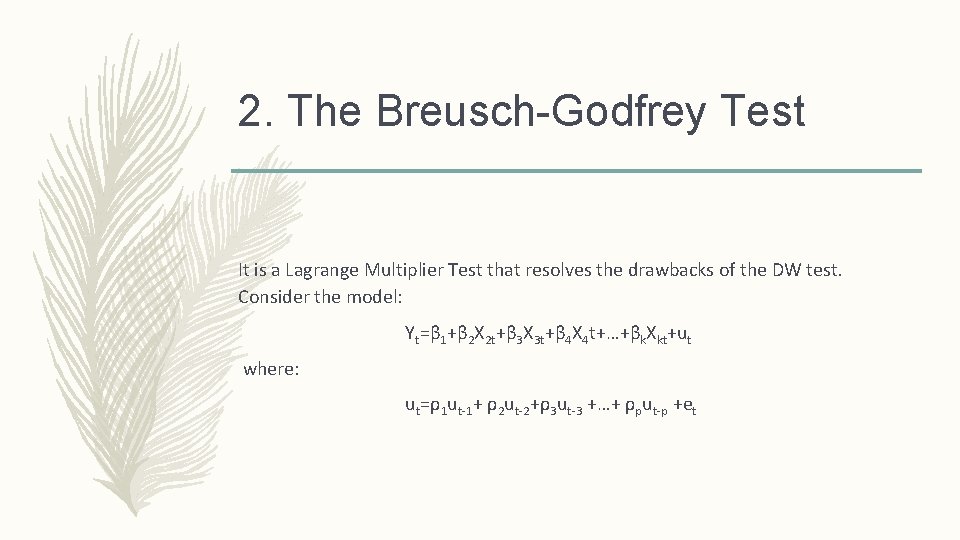
2. The Breusch-Godfrey Test It is a Lagrange Multiplier Test that resolves the drawbacks of the DW test. Consider the model: Yt=β 1+β 2 X 2 t+β 3 X 3 t+β 4 X 4 t+…+βk. Xkt+ut where: ut=ρ1 ut-1+ ρ2 ut-2+ρ3 ut-3 +…+ ρput-p +et

Continue… Combining those two we get: Yt=β 1+β 2 X 2 t+β 3 X 3 t+β 4 X 4 t+…+βk. Xkt+ ρ1 ut-1+ ρ2 ut-2+ρ3 ut-3+…+ ρput-p +et The null and the alternative hypotheses are: H 0: no autocorrelation, when ρ1=ρ2 =ρp=0 H 1: There is autocorrelation, when only one is zero.

Drawback of the BG test 1. A drawback of the BG test is that the value of ρ, the length of the lag, can not be specified a priori. 2. Some experimentation with the ρ value is inevitable. 3. Sometimes one can use the so-called Akaike and Schwarz information criteria to select the lag length.

3. The Durbin’s h Test When there are lagged dependent variables (i. e. Yt-1) then the DW test is not applicable. Durbin developed an alternative test statistic, named the h-statistic, which is calculated by: Where sigma of gamma hat square is the variance of the estimated coefficient of the lagged dependent variable. This statistic is distributed following the normal distribution.

Remedies of Autocorrelation § In first we try to find out if the autocorrelation is pure autocorrelation and not the result of mis-specification of the model. Sometimes we observe patterns in residuals because the model is mis-specified that is it has excluded some important variables or because its functional form is incorrect

Remedies. . § In the case of heteroscedasticity, we will have to use Generalized least square(GLS) method. § If it is pure autocorrelation, one can use appropriate transformation of the original model so that in the transformed model we do not have the problem of pure autocorrelation.

Remedies… Ø When ρ is known, we could use a GLS procedures. e. g. Cochrane-Orcutt Ø When ρ is unknown, we follow some steps. I. Estimate the regression and obtain residuals. II. Estimate autocorrelation from regressing the residual to its lagged terms.

Remedies… Iii- Transform the original variables as starred variable using the obtained from step(ii). iv- Run the regression again with the transformed variables and obtain residuals. v- Continue to repeating step (ii) to (iv) several rounds until the estimate of from two successive iterations differ by no more than some preselected small value such as 0. 001.

Remedies. . § if we find autocorrelation in an application, § we observed to take care of it, for depending on its severity, we may be drawing misleading conclusions because the usual OLS standard errors could be severely biased. Now the problem we face is that we do not know the correlation structure error terms, since they are not directly observable. § In large samples, we can use the Newey-West method to obtain standard errors of OLS estimators that are corrected for autocorrelation. this method is actually an extension of White's heteroscedasticity-consistent standard errors methods. § Some while we can use the OLS method.