Prerequisites Almost essential Welfare and Efficiency PUBLIC GOODS
Prerequisites Almost essential Welfare and Efficiency PUBLIC GOODS MICROECONOMICS Principles and Analysis Frank Cowell April 2018 Frank Cowell: Public Goods 1
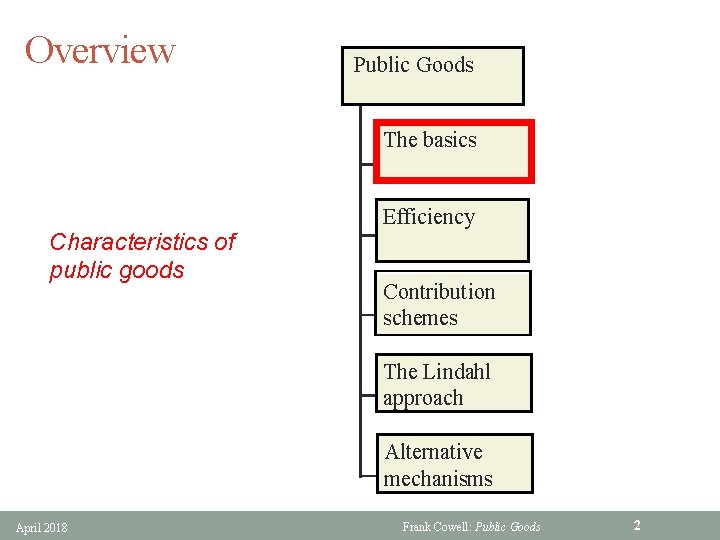
Overview Public Goods The basics Characteristics of public goods Efficiency Contribution schemes The Lindahl approach Alternative mechanisms April 2018 Frank Cowell: Public Goods 2
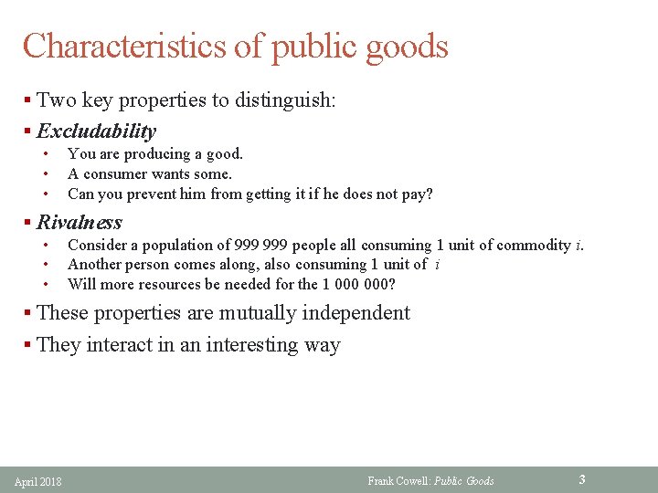
Characteristics of public goods § Two key properties to distinguish: § Excludability • • • You are producing a good. A consumer wants some. Can you prevent him from getting it if he does not pay? § Rivalness • • • Consider a population of 999 people all consuming 1 unit of commodity i. Another person comes along, also consuming 1 unit of i Will more resources be needed for the 1 000? § These properties are mutually independent § They interact in an interesting way April 2018 Frank Cowell: Public Goods 3
![Typology of goods: classic definitions Rival? Excludable? [ Yes ] April 2018 [ Yes Typology of goods: classic definitions Rival? Excludable? [ Yes ] April 2018 [ Yes](http://slidetodoc.com/presentation_image_h2/c960f014deeb984f66a4cb396644eba4/image-4.jpg)
Typology of goods: classic definitions Rival? Excludable? [ Yes ] April 2018 [ Yes ] [ No ] pure private [? ? ] [ No ] [? ? ] pure public Frank Cowell: Public Goods 4
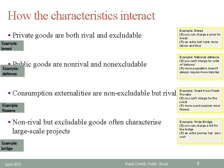
How the characteristics interact § Private goods are both rival and excludable Example: bread § Public goods are nonrival and nonexcludable Example: defence § Consumption externalities are non-excludable but rival Example: flowers § Non-rival but excludable goods often characterise large-scale projects Example: Bread (E) you can charge a price for bread (R) an extra loaf costs more labour and flour Example: National defence (E) you can't charge for units of 'defence‘ (R) more population doesn't always require more missiles Example: Scent from Fresh Flowers (E) you can't charge for the scent (R) more scent requires more flowers Example: Wide Bridge (E) you can charge a toll for the bridge (R) an extra journey has zero cost Example: bridge April 2018 Frank Cowell: Public Goods 5
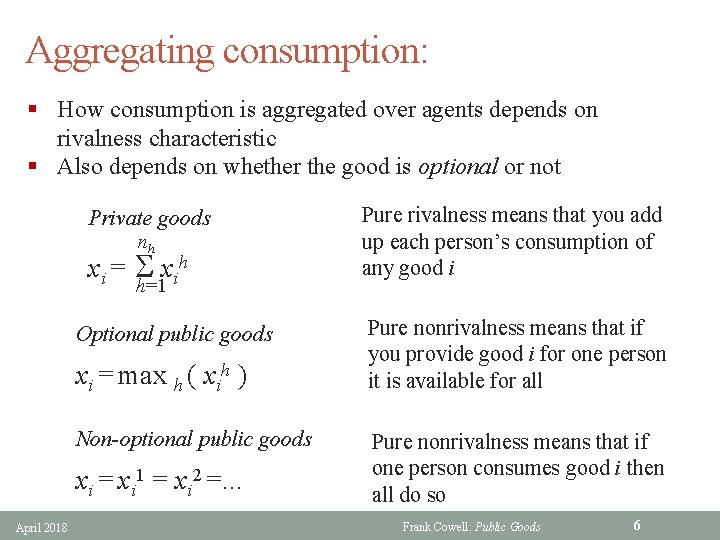
Aggregating consumption: § How consumption is aggregated over agents depends on rivalness characteristic § Also depends on whether the good is optional or not Private goods nh x i = x ih h=1 Optional public goods xi = max h ( xih ) Non-optional public goods xi = xi 1 = xi 2 =. . . April 2018 Pure rivalness means that you add up each person’s consumption of any good i Pure nonrivalness means that if you provide good i for one person it is available for all Pure nonrivalness means that if one person consumes good i then all do so Frank Cowell: Public Goods 6
Overview Public Goods The basics Extending the results that characterise efficient allocations Efficiency Contribution schemes The Lindahl approach Alternative mechanisms April 2018 Frank Cowell: Public Goods 7
Public goods and efficiency § Take the problem of efficient allocation with public goods § The two principal subproblems will be treated separately • characterisation • implementation § Implementation will be treated later § Characterisation can be treated by introducing public-goods characteristics into standard efficiency model April 2018 Frank Cowell: Public Goods 8
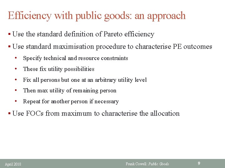
Efficiency with public goods: an approach § Use the standard definition of Pareto efficiency § Use standard maximisation procedure to characterise PE outcomes • Specify technical and resource constraints • These fix utility possibilities • Fix all persons but one at an arbitrary utility level • Then max utility of remaining person • Repeat for another person if necessary § Use FOCs from maximum to characterise the allocation April 2018 Frank Cowell: Public Goods 9
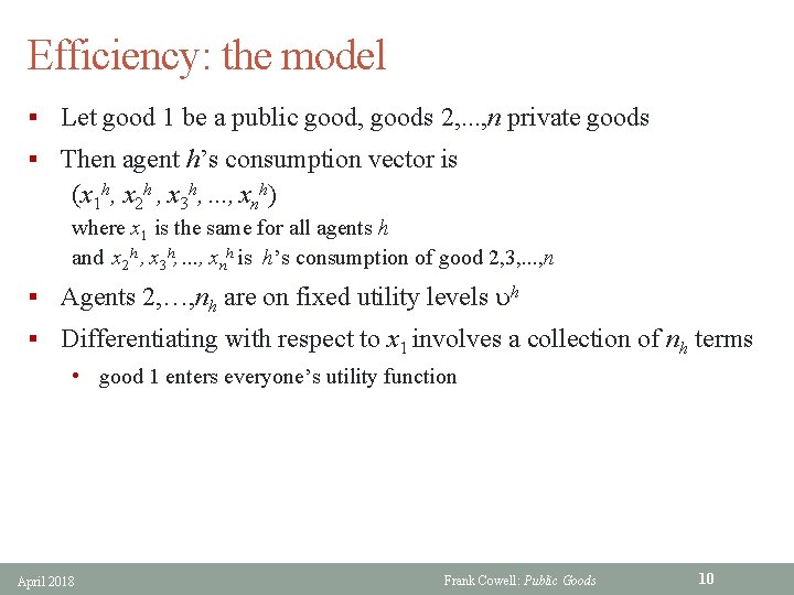
Efficiency: the model § Let good 1 be a public good, goods 2, . . . , n private goods § Then agent h’s consumption vector is (x 1 h, x 2 h , x 3 h, . . . , xnh) where x 1 is the same for all agents h and x 2 h , x 3 h, . . . , xnh is h’s consumption of good 2, 3, . . . , n § Agents 2, …, nh are on fixed utility levels uh § Differentiating with respect to x 1 involves a collection of nh terms • good 1 enters everyone’s utility function April 2018 Frank Cowell: Public Goods 10
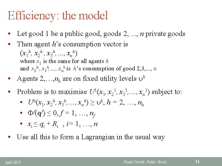
Efficiency: the model § Let good 1 be a public good, goods 2, . . . , n private goods § Then agent h’s consumption vector is (x 1 h, x 2 h , x 3 h, . . . , xnh) where x 1 is the same for all agents h and x 2 h , x 3 h, . . . , xnh is h’s consumption of good 2, 3, . . . , n § Agents 2, …, nh are on fixed utility levels uh § Problem is to maximise U 1(x 1, x 21, x 31, . . . , xn 1) subject to: • Uh(x 1, x 2 h, x 3 h, . . . , xnh) ≥ uh, h = 2, …, nh • Ff(qf) ≤ 0, f = 1, …, nf • xi ≤ qi + Ri , i= 1, …, n § Use all this to form a Lagrangian in the usual way April 2018 Frank Cowell: Public Goods 11
![Finding an efficient allocation max L( [x ], [q], l, m, k) : = Finding an efficient allocation max L( [x ], [q], l, m, k) : =](http://slidetodoc.com/presentation_image_h2/c960f014deeb984f66a4cb396644eba4/image-12.jpg)
Finding an efficient allocation max L( [x ], [q], l, m, k) : = Lagrange multiplier for each utility constraint U 1(x 1) + åhlh [Uh(xh) uh] åf mf F f (q f) Lagrange multiplier for each firm’s technology + åi ki[qi + Ri xi] where Lagrange multiplier for materials balance, good i xh = (x 1, x 2 h, x 3 h, . . . , xnh) xi = åh xih , i = 2, . . . , n qi = åf qi f April 2018 Frank Cowell: Public Goods 12
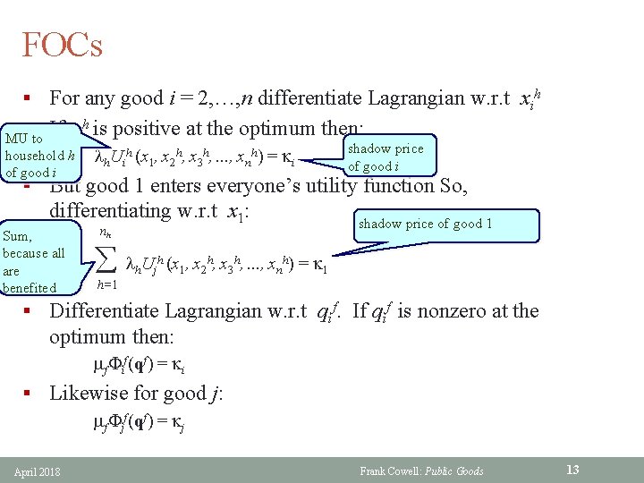
FOCs § For any good i = 2, …, n differentiate Lagrangian w. r. t xih § If x h is positive at the optimum then: shadow price lh. Uih (x 1, x 2 h, x 3 h, . . . , xnh) = ki of good i i MU to household h of good i § But good 1 enters everyone’s utility function So, differentiating w. r. t x 1: Sum, because all are benefited shadow price of good 1 nh å l. U h h h j (x 1, x 2 , x 3 , . . . , xn ) = k 1 h=1 § Differentiate Lagrangian w. r. t qif. If qif is nonzero at the optimum then: mf. Fif(qf) = ki § Likewise for good j: mf. Fjf(qf) = kj April 2018 Frank Cowell: Public Goods 13
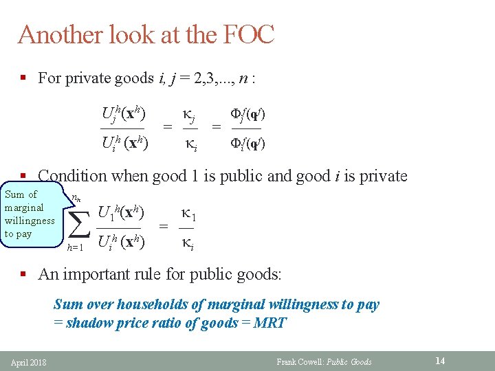
Another look at the FOC § For private goods i, j = 2, 3, . . . , n : Ujh(xh) kj Fjf(qf) ——— = —— Uih (xh) ki Fif(qf) § Condition when good 1 is public and good i is private Sum of marginal willingness to pay nh å h=1 U 1 h(xh) k 1 ——— = — Uih (xh) ki § An important rule for public goods: Sum over households of marginal willingness to pay = shadow price ratio of goods = MRT April 2018 Frank Cowell: Public Goods 14
Overview Public Goods The basics Private provision of public goods? Efficiency Contribution schemes The Lindahl approach Alternative mechanisms April 2018 Frank Cowell: Public Goods 15
The implementation problem § Why is the implementation part of the problem likely to be difficult in the case of pure public goods? § In the general version of the problem private provision will be inefficient § We have an extreme form of the externality issue § We run into the Gibbard-Satterthwaite result April 2018 Frank Cowell: Public Goods 16
Example § Two Goods • good 1 - a pure public good • good 2 - a pure private good § Two persons: A and B • each person has an endowment of good 2 • each contributes to production of good 1 § Production organised in a single firm April 2018 Frank Cowell: Public Goods 17
![Public goods: strategic view (1) §If Alf reneges [–] then Bill’s best response is Public goods: strategic view (1) §If Alf reneges [–] then Bill’s best response is](http://slidetodoc.com/presentation_image_h2/c960f014deeb984f66a4cb396644eba4/image-18.jpg)
Public goods: strategic view (1) §If Alf reneges [–] then Bill’s best response is [–] 2, 2 0, 3 [–] 3, 0 1, 1 [+] [–] §Nash equilibrium Alf [+] §If Bill reneges [–] then Alf’s best response is [–] Bill April 2018 Frank Cowell: Public Goods 18
![Public goods: strategic view (2) §If 1 plays [–] then 2’s best response is Public goods: strategic view (2) §If 1 plays [–] then 2’s best response is](http://slidetodoc.com/presentation_image_h2/c960f014deeb984f66a4cb396644eba4/image-19.jpg)
Public goods: strategic view (2) §If 1 plays [–] then 2’s best response is [+] 2, 2 1, 3 §If 2 plays [+] then 1’s best response is [–] §A Nash equilibrium [–] Alf §By symmetry, another Nash equilibrium 3, 1 0, 0 [+] [–] Bill April 2018 Frank Cowell: Public Goods 19
Which paradigm? § Clearly the two simplified +/– models lead to rather different outcomes § Which is appropriate? Will we inevitably end up at an inefficient outcome? § The answer depends on the technology of production § Also on the number of individuals involved in the community April 2018 Frank Cowell: Public Goods 20
A Voluntary Approach (1) § Consider in detail the implementation problem for public goods § Logical to view the way individual action would work in connection with public goods § Begin with a simple contribution model § Take the case with nh persons § Then see what the “classic” solution would look like April 2018 Frank Cowell: Public Goods 21
A Voluntary Approach (2) § Each person has a fixed endowment of (private) good 2: • R 2 h § And makes a voluntary contribution of some of this toward the production of (public) good 1: • zh = R 2 h – x 2 h § This is equivalent to saying that he chooses to consume this amount of good 2: • x 2 h April 2018 Frank Cowell: Public Goods 22
A Voluntary Approach (3) § Contribution of all households of good 2 is: nh z= z h h=1 § This produces the following amount of good 1: x 1 = f(z) § So the utility payoff to a typical household is: Uh(x 1 , x 2 h) April 2018 Frank Cowell: Public Goods 23
A Voluntary Approach (4) § Suppose every household makes a “Cournot” assumption: nh zk =`z (constant) k=1 k h § Given this and the production function agent h perceives its optimisation problem to be: • max Uh(f(`z + R 2 h – x 2 h ) , x 2 h) § This problem has the first-order condition: • U 1 h(x 1 , x 2 h) fz(`z + R 2 h – x 2 h ) – U 2 h(x 1 , x 2 h) = 0 April 2018 Frank Cowell: Public Goods 24
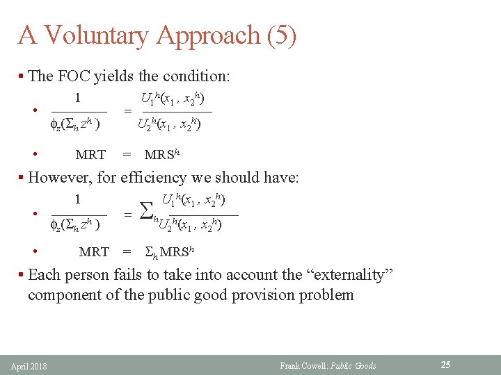
A Voluntary Approach (5) § The FOC yields the condition: 1 U 1 h(x 1 , x 2 h) • ———— = ————— fz( h zh ) U 2 h(x 1 , x 2 h) • MRT = MRSh § However, for efficiency we should have: 1 U 1 h(x 1 , x 2 h) • ———— = h ————— h fz( h z ) U 2 h(x 1 , x 2 h) • MRT = h MRSh § Each person fails to take into account the “externality” component of the public good provision problem April 2018 Frank Cowell: Public Goods 25
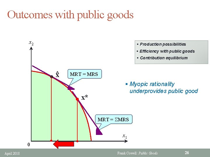
Outcomes with public goods x 2 § Production possibilities § Efficiency with public goods § Contribution equilibrium l ^x MRT = MRS l x* § Myopic rationality underprovides public good MRT = MRS x 1 0 April 2018 Frank Cowell: Public Goods 26
Graphical illustrations § We can use two of the graphical devices that have already proved helpful § The contribution diagram: • Nash outcomes • PE outcomes § The production possibility curve April 2018 Frank Cowell: Public Goods 27
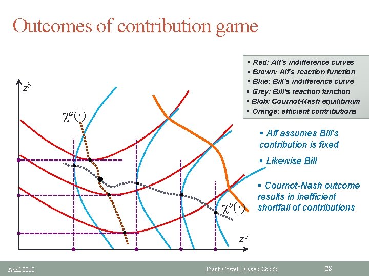
Outcomes of contribution game § Red: Alf’s indifference curves § Brown: Alf’s reaction function § Blue: Bill’s indifference curve § Grey: Bill’s reaction function § Blob: Cournot-Nash equilibrium § Orange: efficient contributions zb ca(·) § Alf assumes Bill’s contribution is fixed § Likewise Bill l l l l April 2018 cb(·) § Cournot-Nash outcome results in inefficient shortfall of contributions za Frank Cowell: Public Goods 28
Overview Public Goods The basics “Personalised” taxes? Efficiency Contribution schemes The Lindahl approach Alternative mechanisms April 2018 Frank Cowell: Public Goods 29
A solution? § Take standard efficiency result for public goods: j MRSj = MRT § This aggregation rule has been used to suggest an allocation mechanism • the “Lindahl solution” is tax-based approach § But the solution is a little unconventional • suggests people should pay taxes according to their willingness to pay • sum of the taxes covers the marginal cost of providing the public good April 2018 Frank Cowell: Public Goods 30
An example § Two Goods • good 1 - a pure public good • good 2 - a pure private good § Two persons: Alf and Bill § Simple organisation of production: A single firm April 2018 Frank Cowell: Public Goods 31
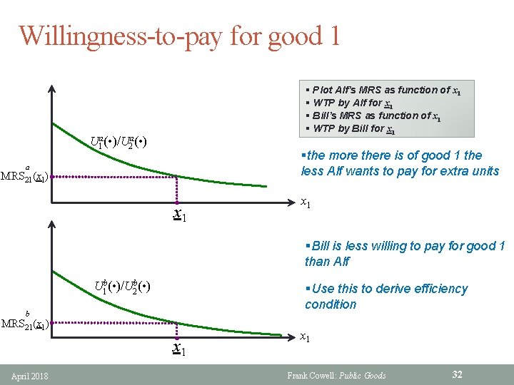
Willingness-to-pay for good 1 § Plot Alf’s MRS as function of x 1 § WTP by Alf for x 1 § Bill’s MRS as function of x 1 § WTP by Bill for x 1 U 1 a( • )/U 2 a( • ) §the more there is of good 1 the less Alf wants to pay for extra units a MRS 21(x 1) x 1 §Bill is less willing to pay for good 1 than Alf U 1 b( • )/U 2 b( • ) §Use this to derive efficiency condition b MRS 21(x 1) x 1 April 2018 x 1 Frank Cowell: Public Goods 32
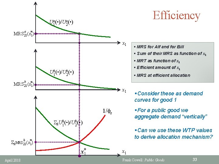
Efficiency Ua 1( • )/Ua 2( • ) a MRS 21(x*1) x 1 § MRS for Alf and for Bill § Sum of their MRS as function of x 1 § MRT as function of x 1 § Efficient amount of x 1 Ub 1( • )/Ub 2( • ) b MRS 21(x*1) § MRS at efficient allocation x 1 §For a public good we aggregate demand “vertically” 1/fz h. Uh 1( • )/U 2 h( • ) §Can we use these WTP values to derive allocation mechanism? h h. MRS 21(x*1) x*1 April 2018 §Consider these as demand curves for good 1 x 1 Frank Cowell: Public Goods 33
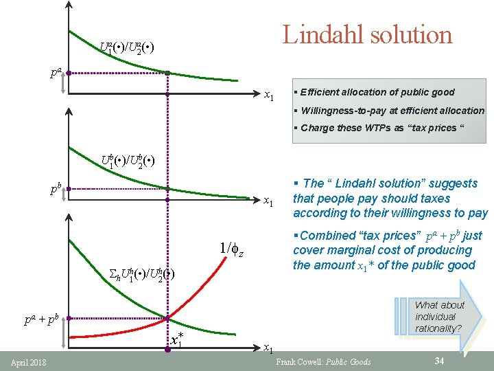
Lindahl solution Ua 1( • )/Ua 2( • ) pa x 1 § Efficient allocation of public good § Willingness-to-pay at efficient allocation § Charge these WTPs as “tax prices “ Ub 1( • )/Ub 2( • ) pb x 1 § The “ Lindahl solution” suggests that people pay should taxes according to their willingness to pay §Combined “tax prices” pa + pb just cover marginal cost of producing the amount x 1* of the public good 1/fz h. Uh 1( • )/U 2 h( • ) What about individual rationality? pa + pb x*1 April 2018 x 1 Frank Cowell: Public Goods 34

The Lindahl Approach § § let ph is the “tax-price” of good 1 for person h, set by the government The FOC for the household’s problem is: 1. § U 1 h(x 1, x 2 h) ———— = ph U 2 h(x 1, x 2 h) For an efficient outcome in terms of the allocation of the two goods: nh 2. p h h=1 § 1 h MRSh = MRT = —— fz(z) Conditions 1, 2 determine set of household-specific prices {ph} April 2018 Frank Cowell: Public Goods 35
The Lindahl Approach (1) § But where does the information come from for this personalised tax-price setting to be implemented? § Presumably from the households themselves § In which case households may view the determination of the personalised prices strategically § In other words h may try to manipulate ph (and thus the allocation) by revealing false information about his MRS April 2018 Frank Cowell: Public Goods 36
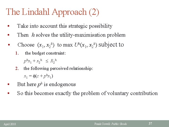
The Lindahl Approach (2) § Take into account this strategic possibility § Then h solves the utility-maximisation problem § Choose (x 1, x 2 h) to max Uh(x 1, x 2 h) subject to 1. the budget constraint: phx 1 + x 2 h R 2 h 2. the following perceived relationship: x 1 = f(c + phx 1) § But here ph is endogenous § So this becomes exactly the problem of voluntary contribution April 2018 Frank Cowell: Public Goods 37
The Way Forward § The Lindahl approach: • results in suboptimal outcome • same as voluntary contribution (subscription) • what can be done? § Public provision through regular taxation § Change the problem § Change perception of the problem April 2018 Frank Cowell: Public Goods 38
Overview Public Goods The basics Truth-revealing devices Efficiency Contribution schemes The Lindahl approach Alternative mechanisms April 2018 Frank Cowell: Public Goods 39
A restricted problem § One reason for the implementation problem: • invite selection of a social state q Q • where Q is large § Sidestep the problem by restricting Q • we would be changing the problem • but in a way that is relevant to many situations § Suppose that there is an all-or nothing choice • replace problem of choosing a specific amount of good 1 from a continuum • substitute the choice problem “select from {NO-PROJECT, PROJECT}” April 2018 Frank Cowell: Public Goods 40
The Clarke-Groves approach § Imagine a project completely characterised by • the status-quo utility • the payment required by each agent if project goes ahead • the utility to each person if it goes ahead § For all individuals • utility is separable • income effect of good 1 is zero: • Uh(x 1 , x 2 h) = y(x 1) + x 2 h April 2018 Frank Cowell: Public Goods 41
The C-G method (2) § Person h has endowment of R 2 h of private good 2 § The project specifies a payment zh for each person conditional on the project going ahead § Total production of good 1 is f(z) where • z : = h zh § Social states Q = {q 0 , q 1} where • q 0 : f(0) = 0 • q 1 : f(z) = 1 § Measure welfare benefit to each h by compensating variation CVh April 2018 Frank Cowell: Public Goods 42
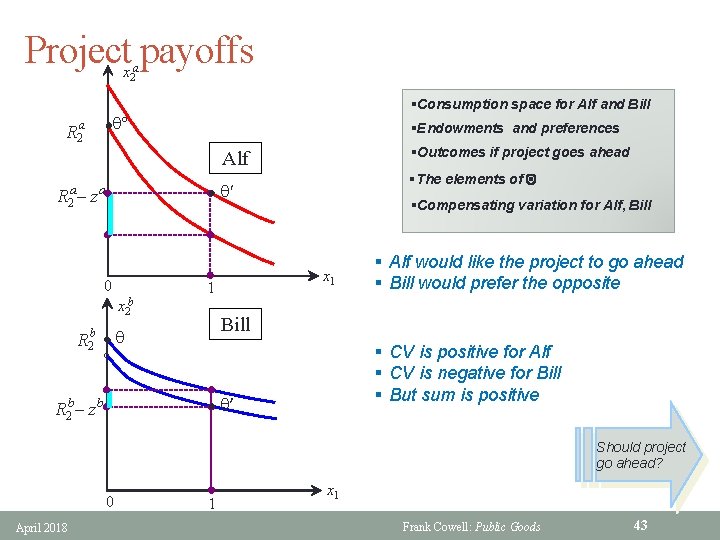
Project payoffs x 2 a §Consumption space for Alf and Bill q° R 2 a §Endowments and preferences l §Outcomes if project goes ahead Alf a R 2 – z a l 0 x 2 b R 2 b l l §The elements of Q q′ §Compensating variation for Alf, Bill x 1 1 Bill q § CV is positive for Alf § CV is negative for Bill § But sum is positive ° R 2 b– z b § Alf would like the project to go ahead § Bill would prefer the opposite l q′ Should project go ahead? 0 April 2018 1 x 1 Frank Cowell: Public Goods 43
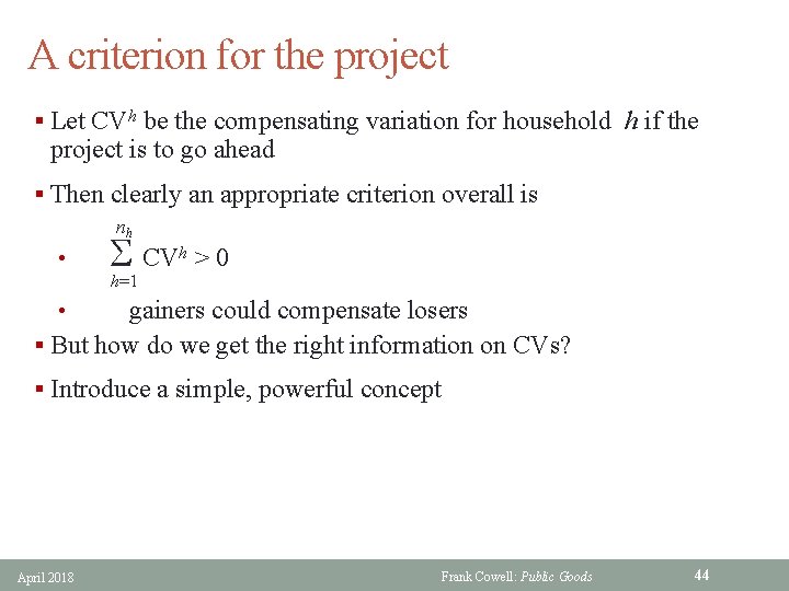
A criterion for the project § Let CVh be the compensating variation for household h if the project is to go ahead § Then clearly an appropriate criterion overall is nh • CVh > 0 h=1 gainers could compensate losers § But how do we get the right information on CVs? • § Introduce a simple, powerful concept April 2018 Frank Cowell: Public Goods 44
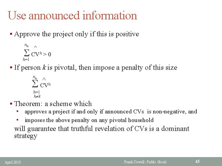
Use announced information § Approve the project only if this is positive nh CVh > 0 h=1 § If person k is pivotal, then impose a penalty of this size nh CV h h=1 h k § Theorem: a scheme which • approves a project if and only if announced CVs is non-negative, and • imposes the above penalty on any pivotal household will guarantee that truthful revelation of CVs is a dominant strategy April 2018 Frank Cowell: Public Goods 45
The pivotal person § Pick an arbitrary person h § What would be the sum of the announced CVs if he were eliminated from the population? § If this sum has the opposite sign from that of the full sum of the CVs, then h is pivotal • adding him swings the result § We use this to construct a mechanism § Consider the following table April 2018 Frank Cowell: Public Goods 46
![Public goods: revelation Everyone else says: [Yes] [No] Decision Nil S forgone gains of Public goods: revelation Everyone else says: [Yes] [No] Decision Nil S forgone gains of](http://slidetodoc.com/presentation_image_h2/c960f014deeb984f66a4cb396644eba4/image-47.jpg)
Public goods: revelation Everyone else says: [Yes] [No] Decision Nil S forgone gains of others [No] S costs §Two possible states §Agent h decision §Payoff table imposed on others Nil An example April 2018 Frank Cowell: Public Goods 47
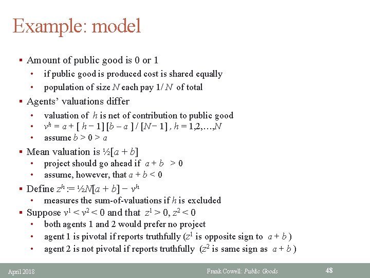
Example: model § Amount of public good is 0 or 1 • • if public good is produced cost is shared equally population of size N each pay 1/ N of total § Agents’ valuations differ • • • valuation of h is net of contribution to public good vh = a + [ h − 1] [b – a ] / [N − 1] , h = 1, 2, …, N assume b > 0 > a § Mean valuation is ½[a + b] • project should go ahead if a + b > 0 • assume, however, that a + b < 0 § Define zh : = ½N[a + b] − vh • measures the sum-of-valuations if h is excluded § Suppose v 1 < v 2 < 0 and that z 1 > 0, z 2 < 0 • both agents 1 and 2 would prefer no project • agent 1 is pivotal if reports truthfully (z 1 is opposite sign to a + b ) • agent 2 is not pivotal if reports truthfully (z 2 is same sign as a + b ) April 2018 Frank Cowell: Public Goods 48
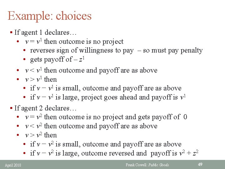
Example: choices § If agent 1 declares… • v = v 1 then outcome is no project • reverses sign of willingness to pay – so must pay penalty • gets payoff of – z 1 • v < v 1 then outcome and payoff are as above • v > v 1 then • if v − v 1 is small, outcome and payoff are as above • if v − v 1 is large, project goes ahead and payoff is v 1 § If agent 2 declares… • v = v 2 then outcome is no project and gets payoff of 0 • v < v 2 then outcome and payoff are as above • v > v 2 then • if v − v 2 is small, outcome and payoff are as above • if v − v 2 is large, outcome reversed and payoff is v 2 + z 2 April 2018 Frank Cowell: Public Goods 49
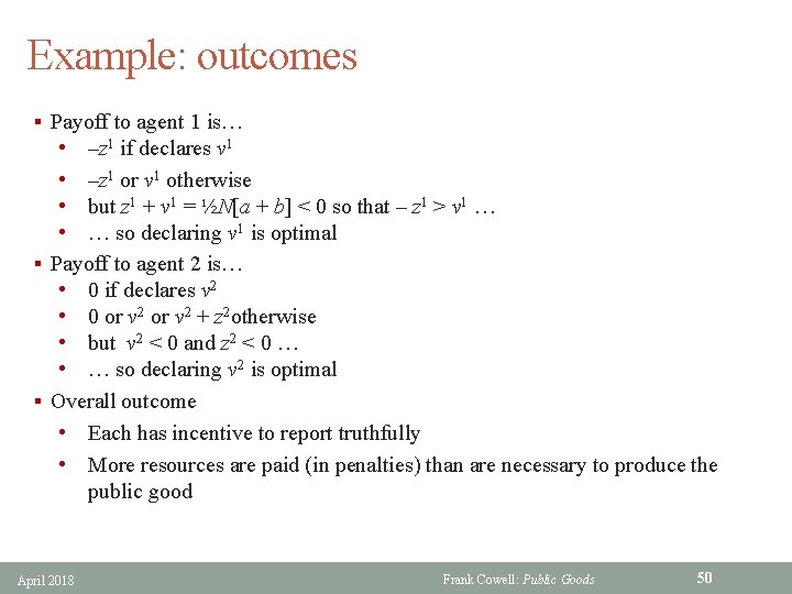
Example: outcomes § Payoff to agent 1 is… • –z 1 if declares v 1 • –z 1 or v 1 otherwise • but z 1 + v 1 = ½N[a + b] < 0 so that – z 1 > v 1 … • … so declaring v 1 is optimal § Payoff to agent 2 is… • 0 if declares v 2 • 0 or v 2 + z 2 otherwise • but v 2 < 0 and z 2 < 0 … • … so declaring v 2 is optimal § Overall outcome • Each has incentive to report truthfully • More resources are paid (in penalties) than are necessary to produce the public good April 2018 Frank Cowell: Public Goods 50
The C-G model – assessment § Strengths: • only uses announced information • elicits truth-telling § Drawbacks: • Restriction to Ziff preferences • Does not ensure budgetary balance § The tipping mechanism can be used as the foundation for more interesting design problems April 2018 Frank Cowell: Public Goods 51
Public goods: summary § Characterisation problem: replace the MRS = MRT rule by S MRS = MRT § Implementation problem: The Lindahl "solution" may not be a solution at all if people can manipulate the system April 2018 Frank Cowell: Public Goods 52
Public goods § The externality feature of public goods makes it easy to solve the characterisation problem § Implementation problems are much harder § Intimately associated with the information problem § Mechanism design depends crucially on the type of public good and the economic environment within which provision is made April 2018 Frank Cowell: Public Goods 53
- Slides: 53