Prerequisites Almost essential Games Mixed Strategies GAMES UNCERTAINTY

Prerequisites Almost essential Games: Mixed Strategies GAMES: UNCERTAINTY MICROECONOMICS Principles and Analysis Frank Cowell April 2018 Frank Cowell: Games Uncertainty 1

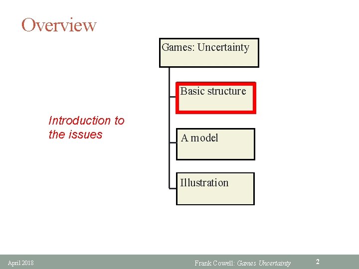
Overview Games: Uncertainty Basic structure Introduction to the issues A model Illustration April 2018 Frank Cowell: Games Uncertainty 2

Introduction § A logical move forward in strategic analysis • follows naturally from considering role of time • similar issues arise concerning the specification of payoffs § Important development • lays the basis for the economics of information • concerns the way in which uncertainty is treated § Connections with analysis of risk-taking • make use of expected utility analysis • but introduce some innovative thinking. April 2018 Frank Cowell: Games Uncertainty 3

Uncertainty § Distinguish from simple randomisation • in principle it is distinct from idea of “mixed strategy” • but see solution method later § Incomplete information • decisions made before features of the game are known • yet players act rationally § Alternative perspective on uncertainty: • an additional player • “nature” makes a move § Role of uncertainty • principally concerns types of player • may know distribution of types • but not the type of any one individual agent April 2018 Frank Cowell: Games Uncertainty 4

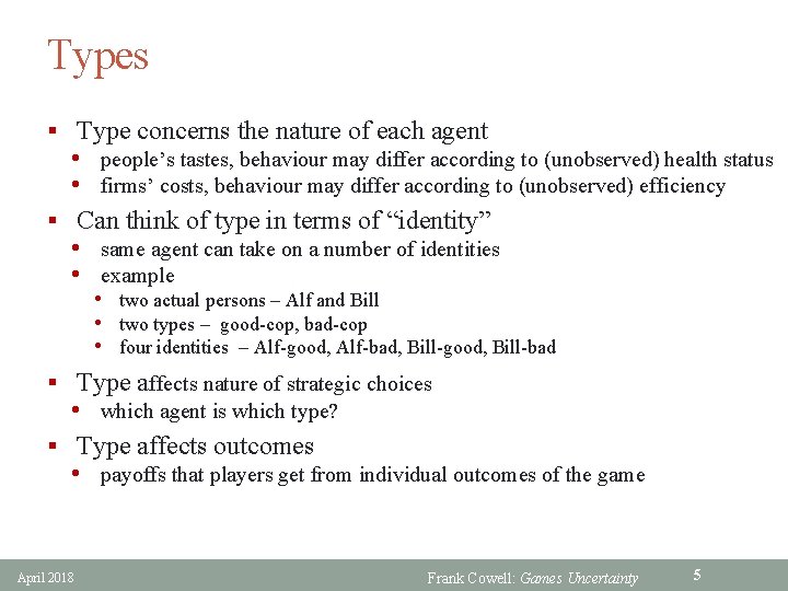
Types § Type concerns the nature of each agent • people’s tastes, behaviour may differ according to (unobserved) health status • firms’ costs, behaviour may differ according to (unobserved) efficiency § Can think of type in terms of “identity” • same agent can take on a number of identities • example • two actual persons – Alf and Bill • two types – good-cop, bad-cop • four identities – Alf-good, Alf-bad, Bill-good, Bill-bad § Type affects nature of strategic choices • which agent is which type? § Type affects outcomes • payoffs that players get from individual outcomes of the game April 2018 Frank Cowell: Games Uncertainty 5

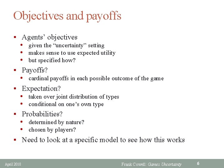
Objectives and payoffs § Agents’ objectives • given the “uncertainty” setting • makes sense to use expected utility • but specified how? § Payoffs? • cardinal payoffs in each possible outcome of the game § Expectation? • taken over joint distribution of types • conditional on one’s own type § Probabilities? • determined by nature? • chosen by players? § Need to look at a specific model to see how this works April 2018 Frank Cowell: Games Uncertainty 6

Overview Games: Uncertainty Basic structure Principles for incorporating uncertainty A model Illustration April 2018 Frank Cowell: Games Uncertainty 7

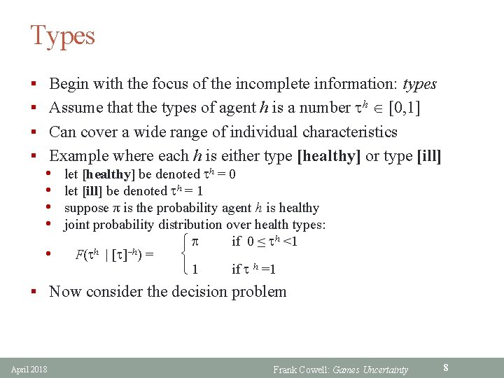
Types § Begin with the focus of the incomplete information: types § Assume that the types of agent h is a number th Î [0, 1] § Can cover a wide range of individual characteristics § Example where each h is either type [healthy] or type [ill] • let [healthy] be denoted th = 0 • let [ill] be denoted th = 1 • suppose π is the probability agent h is healthy • joint probability distribution over health types: p if 0 ≤ th <1 • F(th | [t] h) = 1 if t h =1 § Now consider the decision problem April 2018 Frank Cowell: Games Uncertainty 8

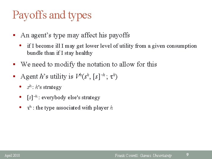
Payoffs and types § An agent’s type may affect his payoffs • if I become ill I may get lower level of utility from a given consumption bundle than if I stay healthy § We need to modify the notation to allow for this § Agent h’s utility is Vh(sh, [s] h ; τh) • sh : h's strategy • [s] h : everybody else's strategy • τh : the type associated with player h April 2018 Frank Cowell: Games Uncertainty 9

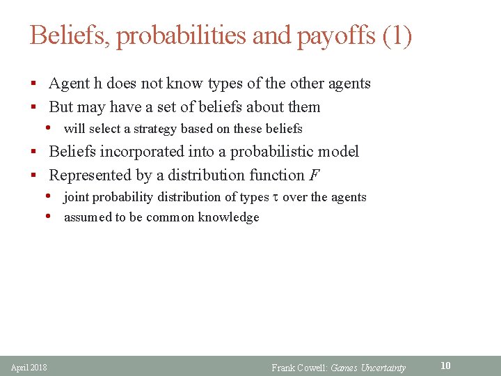
Beliefs, probabilities and payoffs (1) § Agent h does not know types of the other agents § But may have a set of beliefs about them • will select a strategy based on these beliefs § Beliefs incorporated into a probabilistic model § Represented by a distribution function F • joint probability distribution of types t over the agents • assumed to be common knowledge April 2018 Frank Cowell: Games Uncertainty 10

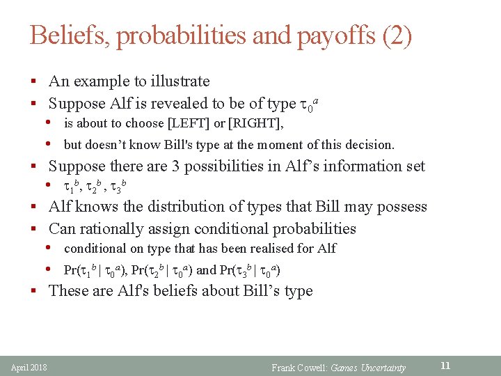
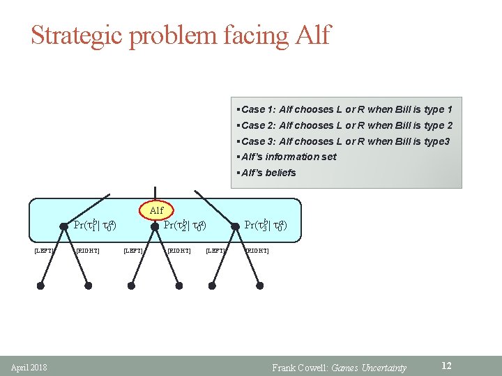
Beliefs, probabilities and payoffs (2) § An example to illustrate § Suppose Alf is revealed to be of type t 0 a • is about to choose [LEFT] or [RIGHT], • but doesn’t know Bill's type at the moment of this decision. § Suppose there are 3 possibilities in Alf’s information set • t 1 b, t 2 b , t 3 b § Alf knows the distribution of types that Bill may possess § Can rationally assign conditional probabilities • conditional on type that has been realised for Alf • Pr(t 1 b | t 0 a), Pr(t 2 b | t 0 a) and Pr(t 3 b | t 0 a) § These are Alf's beliefs about Bill’s type April 2018 Frank Cowell: Games Uncertainty 11

Strategic problem facing Alf §Case 1: Alf chooses L or R when Bill is type 1 §Case 2: Alf chooses L or R when Bill is type 2 §Case 3: Alf chooses L or R when Bill is type 3 §Alf’s information set §Alf’s beliefs Alf Pr(t 1 b| t 0 a) [LEFT] April 2018 [RIGHT] Pr(t 2 b | t 0 a) [LEFT] [RIGHT] [LEFT] Pr(t 3 b | t 0 a) [RIGHT] Frank Cowell: Games Uncertainty 12

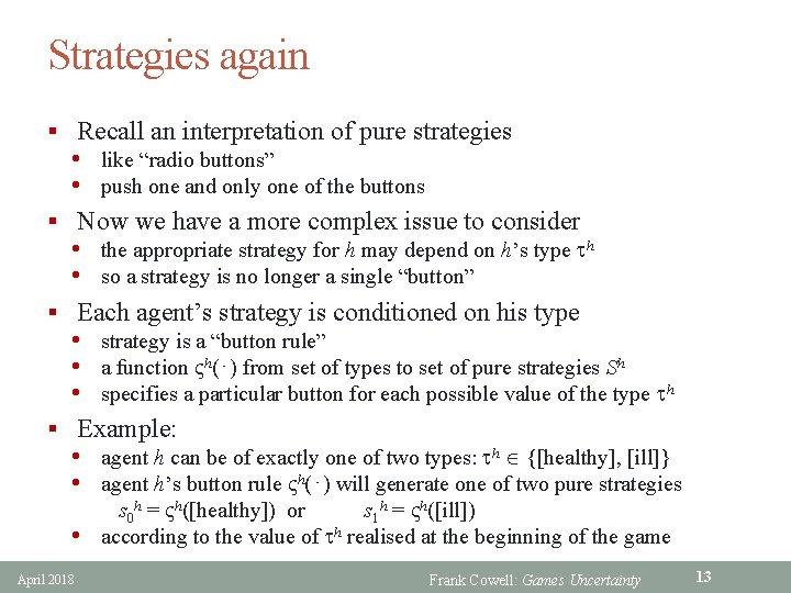
Strategies again § Recall an interpretation of pure strategies • like “radio buttons” • push one and only one of the buttons § Now we have a more complex issue to consider • the appropriate strategy for h may depend on h’s type th • so a strategy is no longer a single “button” § Each agent’s strategy is conditioned on his type • strategy is a “button rule” • a function h(⋅) from set of types to set of pure strategies Sh • specifies a particular button for each possible value of the type th § Example: • agent h can be of exactly one of two types: th Î {[healthy], [ill]} • agent h’s button rule h(⋅) will generate one of two pure strategies s 0 h = h([healthy]) or s 1 h = h([ill]) • according to the value of th realised at the beginning of the game April 2018 Frank Cowell: Games Uncertainty 13

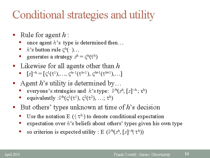
Conditional strategies and utility § Rule for agent h : • once agent h’s type is determined then… • h’s button rule h(⋅)… • generates a strategy sh = h(th) § Likewise for all agents other than h • [s] h = [ 1(t 1), …, h 1(th 1), h+1(th+1), …] § Agent h’s utility is determined by… • everyone’s strategies and h’s type: Vh(sh, [s] h ; τh) • equivalently : Vh( 1(t 1), 2(t 2), …; th) § But others’ types unknown at time of h’s decision • Use the notation E (∙| th ) to denote conditional expectation • expectation over h’s beliefs about others’ types given his own type • so criterion is expected utility : E (Vh(sh, [s] h| th)) April 2018 Frank Cowell: Games Uncertainty 14

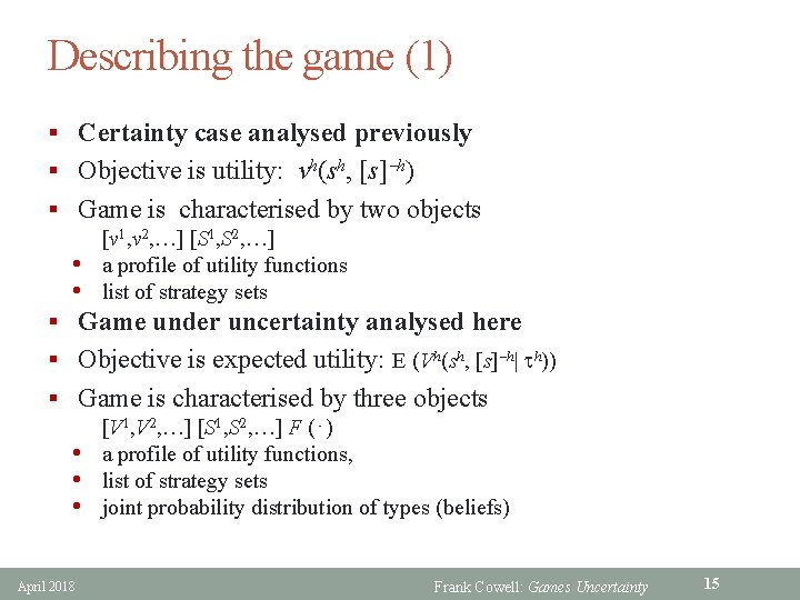
Describing the game (1) § Certainty case analysed previously § Objective is utility: vh(sh, [s] h) § Game is characterised by two objects [v 1, v 2, …] [S 1, S 2, …] • a profile of utility functions • list of strategy sets § Game under uncertainty analysed here § Objective is expected utility: E (Vh(sh, [s] h| th)) § Game is characterised by three objects [V 1, V 2, …] [S 1, S 2, …] F (⋅) • a profile of utility functions, • list of strategy sets • joint probability distribution of types (beliefs) April 2018 Frank Cowell: Games Uncertainty 15

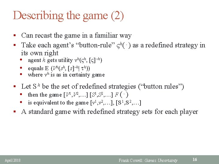
Describing the game (2) § Can recast the game in a familiar way § Take each agent’s “button-rule” h(⋅) as a redefined strategy in its own right • agent h gets utility vh( h, [ ] h) • equals E (Vh(sh, [s] h| th)) • where vh is as in certainty game § Let S h be the set of redefined strategies (“button rules”) • then the game [V 1, V 2, …] [S 1, S 2, …] F (⋅) • is equivalent to the game [v 1, v 2, …], [S 1, S 2, …] § A standard game with redefined strategy sets for each player April 2018 Frank Cowell: Games Uncertainty 16

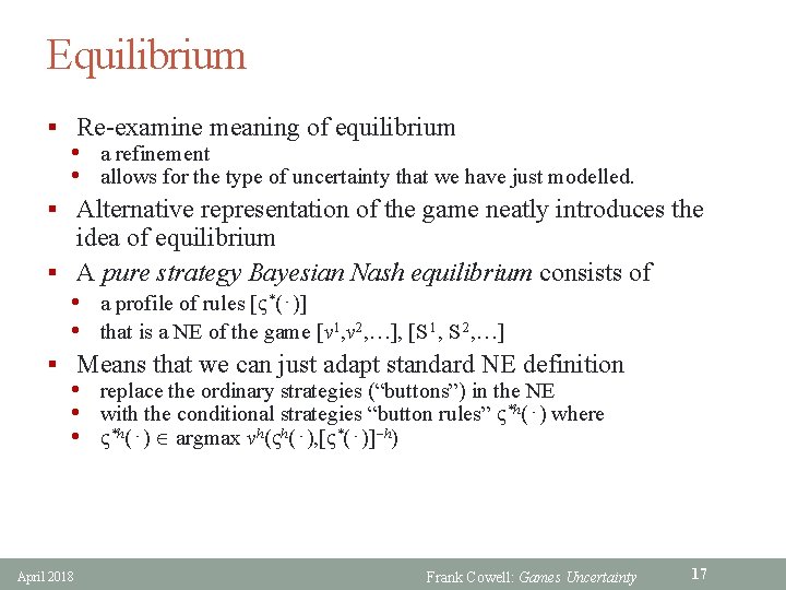
Equilibrium § Re-examine meaning of equilibrium • a refinement • allows for the type of uncertainty that we have just modelled. § Alternative representation of the game neatly introduces the idea of equilibrium § A pure strategy Bayesian Nash equilibrium consists of • a profile of rules [ *(⋅)] • that is a NE of the game [v 1, v 2, …], [S 1, S 2, …] § Means that we can just adapt standard NE definition • replace the ordinary strategies (“buttons”) in the NE • with the conditional strategies “button rules” *h(⋅) where • *h(⋅) Î argmax vh( h(⋅), [ *(⋅)] h) April 2018 Frank Cowell: Games Uncertainty 17

Equilibrium: definition § Definition • A profile of decision rules [ *] is a Bayesian-Nash equilibrium for the game • if and only if for all h and for any t 0 h occurring with positive probability • E(Vh( *h(t 0 h), [s*] h| t 0 h)) ≥ E(Vh(sh, [s*] h| t 0 h)) for all sh Î Sh § Identity interpretation • Bayesian equilibrium as a Nash equilibrium of a game with a larger • • • April 2018 number of players if there are n players and m types this setup as equivalent to a game with mn players Each agent in a particular identity plays to maximise expected utility in that identity Frank Cowell: Games Uncertainty 18

Model: summary § We have extended the standard analysis • objectives • strategies • equilibrium § To allow for case where agents’ types are unknown • everything based on expected values • conditioned on agent’s own type § Let’s put this to work in an example • illustrate equilibrium concept • outline a method of solution April 2018 Frank Cowell: Games Uncertainty 19

Overview Games: Uncertainty Basic structure the entry game (again) A model Illustration April 2018 Frank Cowell: Games Uncertainty 20

Entry game: uncertainty § Connected to previous lectures of strategic issues in industrial organisation § But there’s a new twist • characteristics of firm 1 (the incumbent) • not fully known by firm 2 (an entrant) § Firm 1 can commit to investment • would enhance firm 1's market position • might deter entry § Cost of investment is crucial • firm 1 may be either high cost or low cost • which of these two actually applies is unknown to firm 2 April 2018 Begin with a review of the certainty case Frank Cowell: Games Uncertainty 21

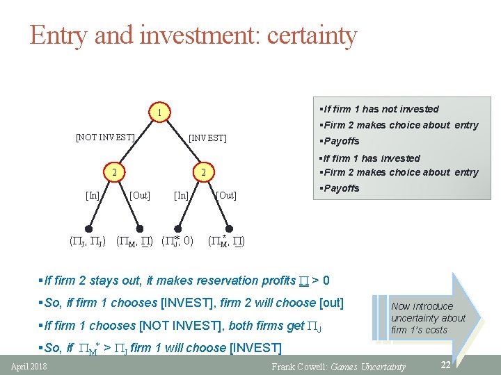
Entry and investment: certainty §If firm 1 has not invested 1 §Firm 2 makes choice about entry [NOT INVEST] [INVEST] 2 [In] §Payoffs §If firm 1 has invested §Firm 2 makes choice about entry 2 [Out] [In] (PJ, PJ) (PM, P) _ (P*J, 0) §Payoffs [Out] (PM*, P) _ §If firm 2 stays out, it makes reservation profits P > 0 §So, if firm 1 chooses [INVEST], firm 2 will choose [out] §If firm 1 chooses [NOT INVEST], both firms get PJ Now introduce uncertainty about firm 1’s costs §So, if PM* > PJ firm 1 will choose [INVEST] April 2018 Frank Cowell: Games Uncertainty 22

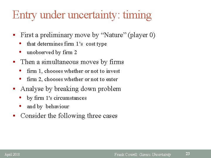
Entry under uncertainty: timing § First a preliminary move by “Nature” (player 0) • that determines firm 1’s cost type • unobserved by firm 2 § Then a simultaneous moves by firms • firm 1, chooses whether or not to invest • firm 2, chooses whether or not to enter § Analyse by breaking down problem • by firm 1's circumstances • and by behaviour § Consider the following three cases April 2018 Frank Cowell: Games Uncertainty 23

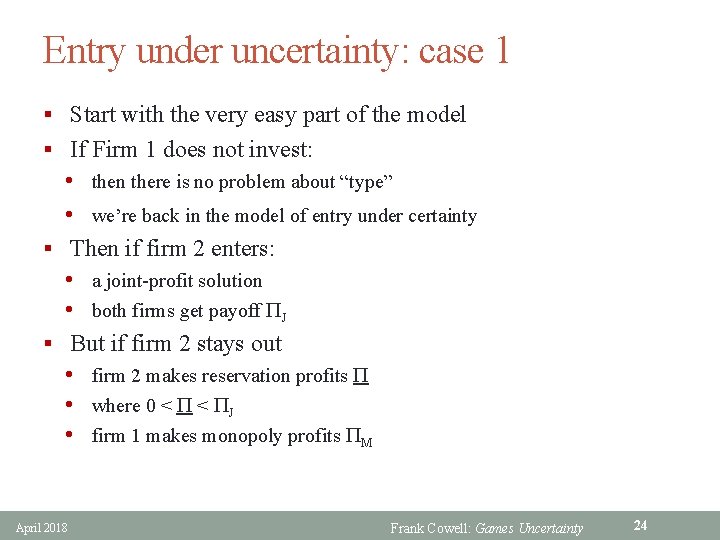
Entry under uncertainty: case 1 § Start with the very easy part of the model § If Firm 1 does not invest: • then there is no problem about “type” • we’re back in the model of entry under certainty § Then if firm 2 enters: • a joint-profit solution • both firms get payoff PJ § But if firm 2 stays out • firm 2 makes reservation profits P • where 0 < PJ • firm 1 makes monopoly profits PM April 2018 Frank Cowell: Games Uncertainty 24

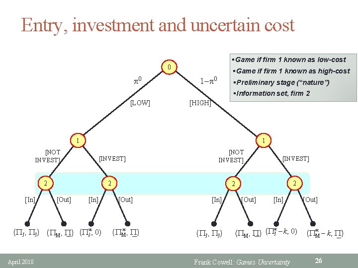
Entry under uncertainty: cases 2, 3 § [2] If Firm 1 invests and is low cost: § Then if firm 2 enters • firm 1 makes profits PJ* < PJ • firm 2's profits are forced to zero § But if firm 2 stays out • firm 1 gets enhanced monopoly profits PM* > PM • firm 2 gets reservation profits P § [3] If Firm 1 invests and is high cost: § Then if firm 2 enters • firm 1 makes profits PJ* − k (where k > 0) • firm 2's profits are forced to zero § But if firm 2 stays out • firm 1 gets enhanced monopoly profits PM* − k • firm 2 gets reservation profits P April 2018 Now assemble all this in a diagram Frank Cowell: Games Uncertainty 25

Entry, investment and uncertain cost §Game if firm 1 known as low-cost 0 p 0 §Game if firm 1 known as high-cost 1 p 0 §Preliminary stage (“nature”) §Information set, firm 2 [LOW] [HIGH] 1 [NOT INVEST] 1 [INVEST] 2 [In] [INVEST] 2 2 2 [Out] [In] (PJ, PJ) (PM, P) _ (P*J, 0) April 2018 [NOT INVEST] [Out] * , P) (PM _ [In] (PJ, PJ) [Out] [In] _ (P*J – k, 0) (PM, P) Frank Cowell: Games Uncertainty [Out] (P*M – k, P) _` 26

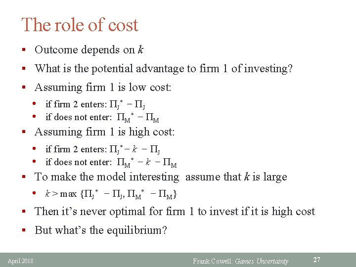
The role of cost § Outcome depends on k § What is the potential advantage to firm 1 of investing? § Assuming firm 1 is low cost: • if firm 2 enters: PJ* − PJ • if does not enter: PM* − PM § Assuming firm 1 is high cost: • if firm 2 enters: PJ* − k − PJ • if does not enter: PM* − k − PM § To make the model interesting assume that k is large • k > max {PJ* − PJ, PM* − PM} § Then it’s never optimal for firm 1 to invest if it is high cost § But what’s the equilibrium? April 2018 Frank Cowell: Games Uncertainty 27

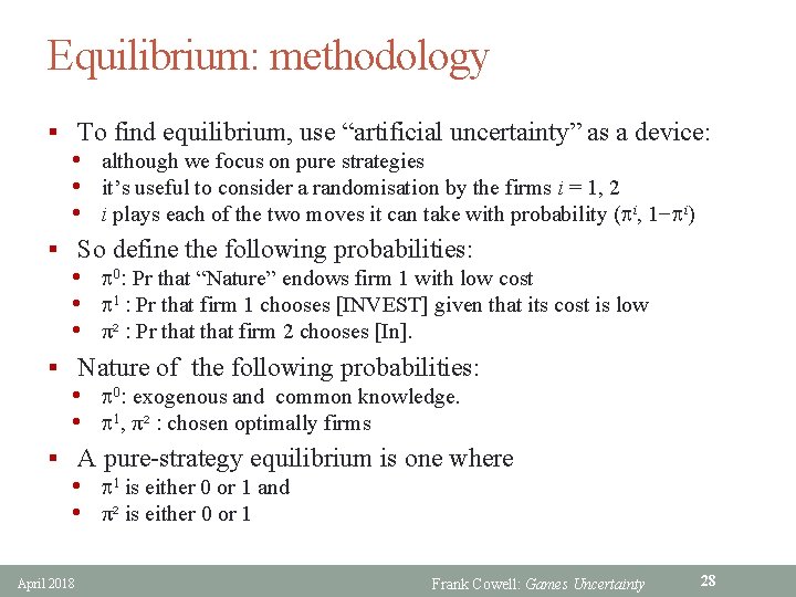
Equilibrium: methodology § To find equilibrium, use “artificial uncertainty” as a device: • although we focus on pure strategies • it’s useful to consider a randomisation by the firms i = 1, 2 • i plays each of the two moves it can take with probability (pi, 1−pi) § So define the following probabilities: • p 0: Pr that “Nature” endows firm 1 with low cost • p 1 : Pr that firm 1 chooses [INVEST] given that its cost is low • π² : Pr that firm 2 chooses [In]. § Nature of the following probabilities: • p 0: exogenous and common knowledge. • p 1, π² : chosen optimally firms § A pure-strategy equilibrium is one where • p 1 is either 0 or 1 and • π² is either 0 or 1 April 2018 Frank Cowell: Games Uncertainty 28

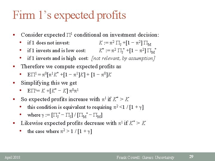
Firm 1’s expected profits Consider expected P 1 conditional on investment decision: § • if 1 does not invest: K : = p 2 PJ +[1 − p 2] PM • if 1 invests and is low cost: K* : = p 2 PJ* +[1 − p 2] PM* • if 1 invests and is high cost: [not relevant, by assumption] Therefore we compute expected profits as § • EP 1 = p 0[p 1 K* +[1 − p 1]K] + [1 − p 0]K Simplifying this we get § • EP¹= K +[K* − K] p 0 p 1 So expected profits increase with p 1 if K* > K § • this condition is equivalent to requiring p 2 <1 / [1 + g] • where g : = [PJ* − PJ] / [PM* − PM] Likewise expected profits decrease with p 1 if K* > K § • the case where p 2 > 1 / [1 + g] April 2018 Frank Cowell: Games Uncertainty 29

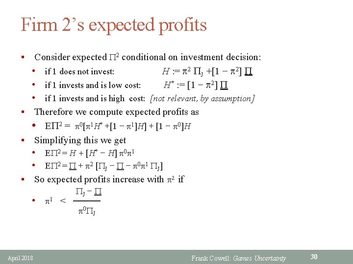
Firm 2’s expected profits § Consider expected P 2 conditional on investment decision: • if 1 does not invest: H : = p 2 PJ +[1 − p 2] P • if 1 invests and is low cost: H* : = [1 − p 2] P • if 1 invests and is high cost: [not relevant, by assumption] Therefore we compute expected profits as • EP 2 = p 0[p 1 H* +[1 − p 1]H] + [1 − p 0]H § Simplifying this we get § • EP 2 = H + [H* − H] p 0 p 1 • EP 2 = P + p 2 [PJ − P − p 0 p 1 PJ] So expected profits increase with p 2 if § PJ − P • p 1 < ──── p 0 PJ April 2018 Frank Cowell: Games Uncertainty 30

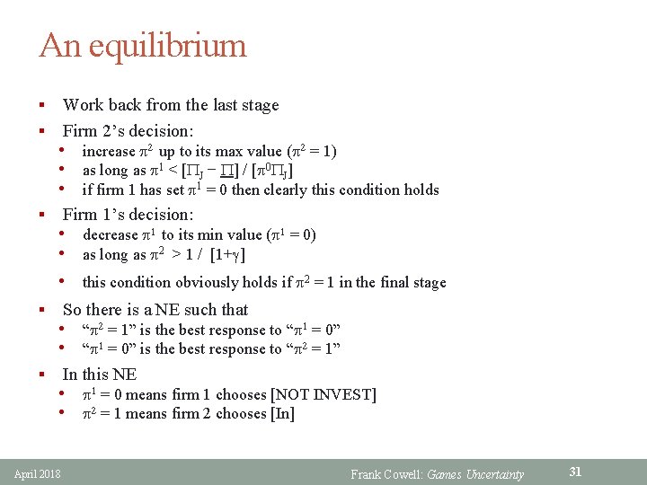
An equilibrium Work back from the last stage § Firm 2’s decision: § • increase p 2 up to its max value (p 2 = 1) • as long as p 1 < [PJ − P] / [p 0 PJ] • if firm 1 has set p 1 = 0 then clearly this condition holds § § § Firm 1’s decision: • decrease p 1 to its min value (p 1 = 0) • as long as p 2 > 1 / [1+g] • this condition obviously holds if p 2 = 1 in the final stage So there is a NE such that • “p 2 = 1” is the best response to “p 1 = 0” • “p 1 = 0” is the best response to “p 2 = 1” In this NE • p 1 = 0 means firm 1 chooses [NOT INVEST] • p 2 = 1 means firm 2 chooses [In] April 2018 Frank Cowell: Games Uncertainty 31

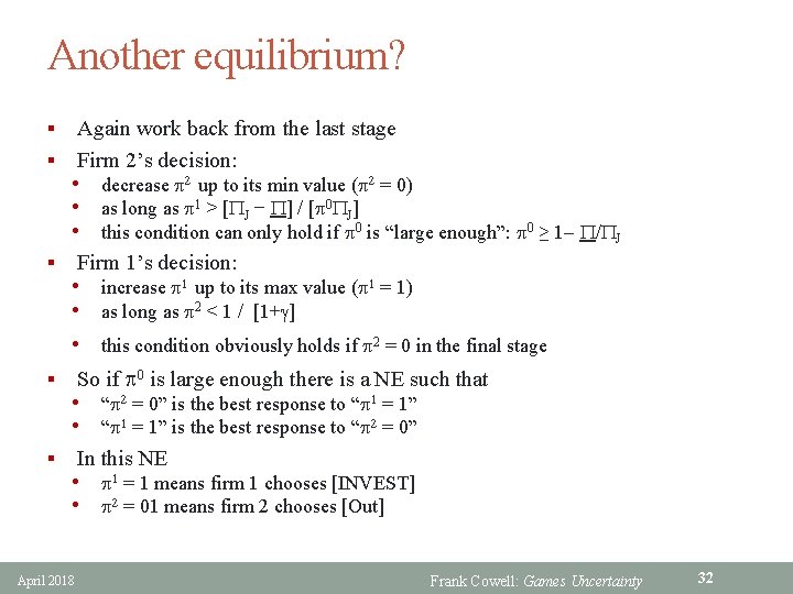
Another equilibrium? Again work back from the last stage § Firm 2’s decision: § • decrease p 2 up to its min value (p 2 = 0) • as long as p 1 > [PJ − P] / [p 0 PJ] • this condition can only hold if p 0 is “large enough”: p 0 ≥ 1 P/PJ § § § Firm 1’s decision: • increase p 1 up to its max value (p 1 = 1) • as long as p 2 < 1 / [1+g] • this condition obviously holds if p 2 = 0 in the final stage So if p 0 is large enough there is a NE such that • “p 2 = 0” is the best response to “p 1 = 1” • “p 1 = 1” is the best response to “p 2 = 0” In this NE • p 1 = 1 means firm 1 chooses [INVEST] • p 2 = 01 means firm 2 chooses [Out] April 2018 Frank Cowell: Games Uncertainty 32

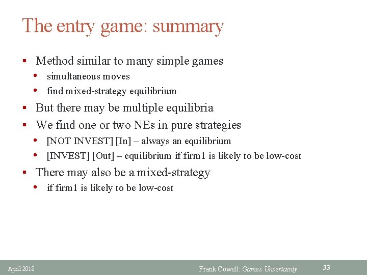
The entry game: summary § Method similar to many simple games • simultaneous moves • find mixed-strategy equilibrium § But there may be multiple equilibria § We find one or two NEs in pure strategies • [NOT INVEST] [In] – always an equilibrium • [INVEST] [Out] – equilibrium if firm 1 is likely to be low-cost § There may also be a mixed-strategy • if firm 1 is likely to be low-cost April 2018 Frank Cowell: Games Uncertainty 33

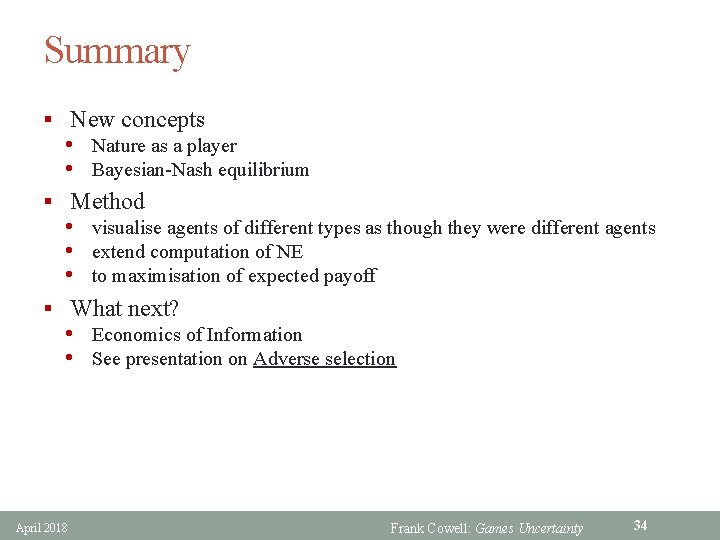
Summary § New concepts • Nature as a player • Bayesian-Nash equilibrium § Method • visualise agents of different types as though they were different agents • extend computation of NE • to maximisation of expected payoff § What next? • Economics of Information • See presentation on Adverse selection April 2018 Frank Cowell: Games Uncertainty 34