Prerequisites Almost essential Firm Optimisation THE FIRM DEMAND

Prerequisites Almost essential Firm: Optimisation THE FIRM: DEMAND SUPPLY MICROECONOMICS Principles and Analysis Frank Cowell April 2018 Frank Cowell: Firm- Demand & Supply 1

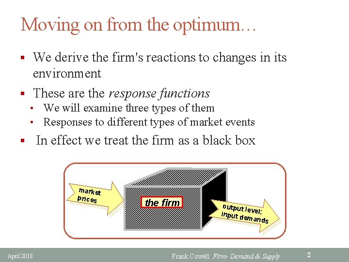
Moving on from the optimum… § We derive the firm's reactions to changes in its environment § These are the response functions • We will examine three types of them • Responses to different types of market events § In effect we treat the firm as a black box market prices April 2018 the firm output level; input d emands Frank Cowell: Firm- Demand & Supply 2

The firm as a “black box” § Behaviour can be predicted by necessary and sufficient conditions for optimum § The FOC can be solved to yield behavioural response functions § Their properties derive from the solution function • • April 2018 we need the solution function’s properties apply them again and again Frank Cowell: Firm- Demand & Supply 3

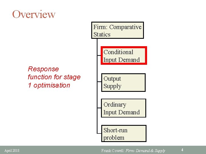
Overview Firm: Comparative Statics Conditional Input Demand Response function for stage 1 optimisation Output Supply Ordinary Input Demand Short-run problem April 2018 Frank Cowell: Firm- Demand & Supply 4

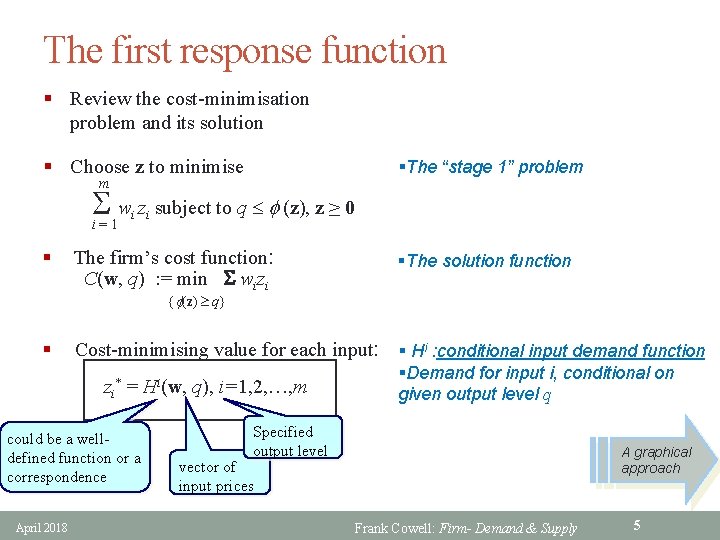
The first response function § Review the cost-minimisation problem and its solution § Choose z to minimise §The “stage 1” problem m S wi zi subject to q f (z), z ≥ 0 i=1 § The firm’s cost function: C(w, q) : = min S wizi §The solution function {f(z) ³ q} § Cost-minimising value for each input: § Hi : conditional input demand function zi* = could be a welldefined function or a correspondence April 2018 Hi(w, q), i=1, 2, …, m §Demand for input i, conditional on given output level q Specified output level A graphical approach vector of input prices Frank Cowell: Firm- Demand & Supply 5

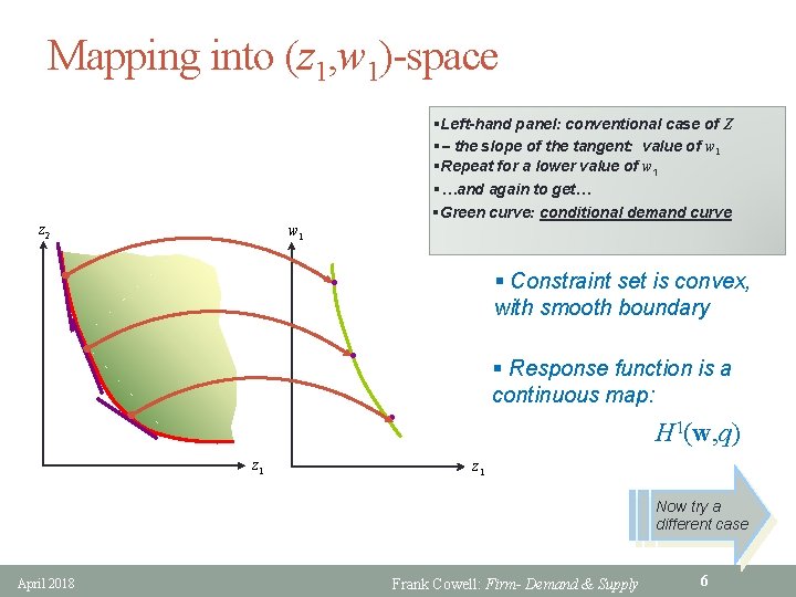
Mapping into (z 1, w 1)-space §Left-hand panel: conventional case of Z § the slope of the tangent: value of w 1 §Repeat for a lower value of w 1 §…and again to get… §Green curve: conditional demand curve z 2 w 1 § Constraint set is convex, with smooth boundary l l § Response function is a continuous map: l z 1 H 1(w, q) z 1 Now try a different case April 2018 Frank Cowell: Firm- Demand & Supply 6

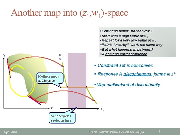
Another map into (z 1, w 1)-space z 2 §Left-hand panel: nonconvex Z §Start with a high value of w 1 §Repeat for a very low value of w 1 §Points “nearby” `work the same way §But what happens in between? §A demand correspondence w 1 § Constraint set is nonconvex l l § Response is discontinuous: jumps in z* Multiple inputs at this price l l §Map multivalued at discontinuity l l z 1 no price yields a solution here April 2018 Frank Cowell: Firm- Demand & Supply 7

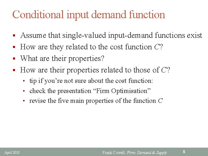
Conditional input demand function § Assume that single-valued input-demand functions exist § How are they related to the cost function C? § What are their properties? § How are their properties related to those of C? • tip if you’re not sure about the cost function: • check the presentation “Firm Optimisation” • revise the five main properties of the function C April 2018 Frank Cowell: Firm- Demand & Supply 8

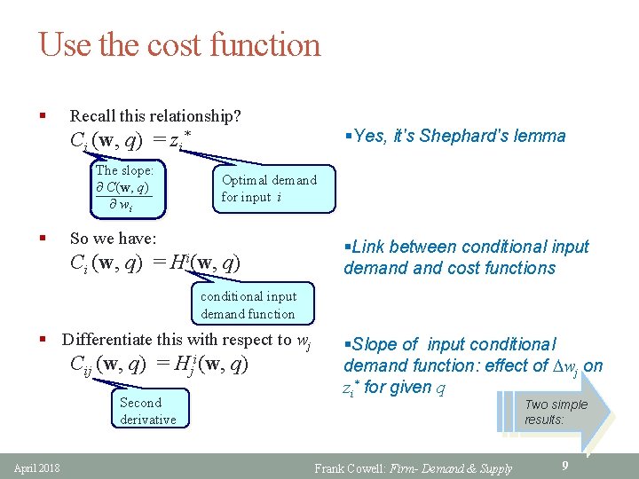
Use the cost function § Recall this relationship? §Yes, it's Shephard's lemma Ci (w, q) = zi* The slope: ¶ C(w, q) ———— ¶ wi § Optimal demand for input i So we have: Ci (w, q) = Hi(w, q) §Link between conditional input demand cost functions conditional input demand function § Differentiate this with respect to wj Cij (w, q) = Hji(w, q) Second derivative April 2018 §Slope of input conditional demand function: effect of Dwj on zi* for given q Two simple results: Frank Cowell: Firm- Demand & Supply 9

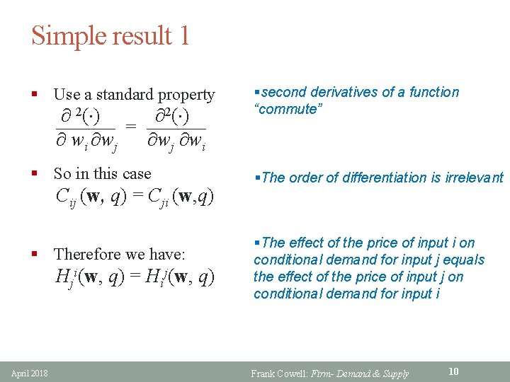
Simple result 1 § Use a standard property §second derivatives of a function “commute” § So in this case §The order of differentiation is irrelevant ¶ 2( ) ——— = ——— ¶ wi ¶wj ¶wi Cij (w, q) = Cji (w, q) § Therefore we have: Hji(w, q) = Hij(w, q) April 2018 §The effect of the price of input i on conditional demand for input j equals the effect of the price of input j on conditional demand for input i Frank Cowell: Firm- Demand & Supply 10

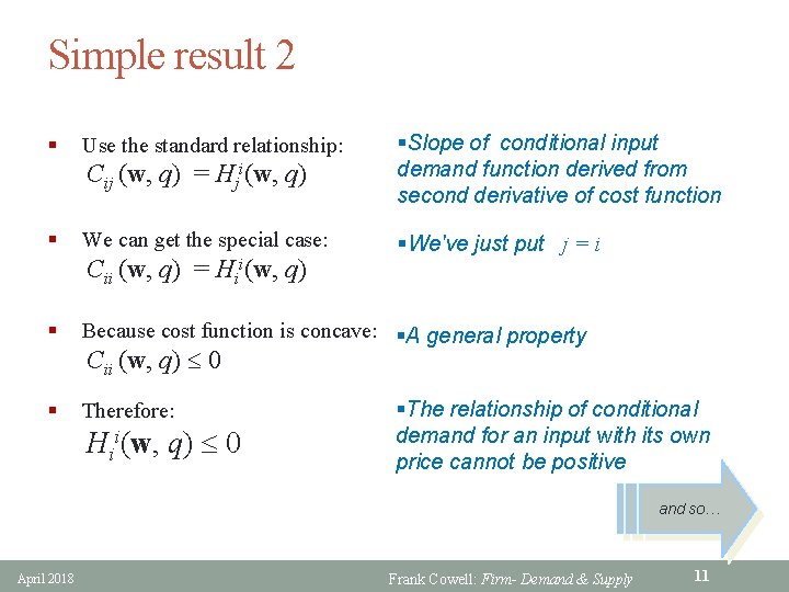
Simple result 2 § § Cij (w, q) = Hji(w, q) §Slope of conditional input demand function derived from second derivative of cost function We can get the special case: §We've just put j = i Use the standard relationship: Cii (w, q) = Hii(w, q) § Because cost function is concave: §A general property § Therefore: Cii (w, q) 0 Hii(w, q) 0 §The relationship of conditional demand for an input with its own price cannot be positive and so… April 2018 Frank Cowell: Firm- Demand & Supply 11

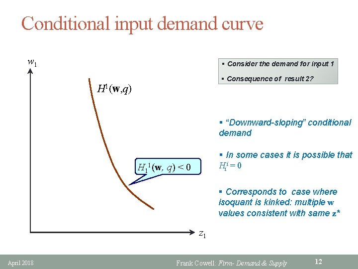
Conditional input demand curve w 1 § Consider the demand for input 1 § Consequence of result 2? H 1(w, q) § “Downward-sloping” conditional demand § In some cases it is possible that Hii = 0 H 11(w, q) < 0 § Corresponds to case where isoquant is kinked: multiple w values consistent with same z* z 1 April 2018 Frank Cowell: Firm- Demand & Supply 12

Conditional demand function: summary § Nonconvex Z yields discontinuous H § Cross-price effects are symmetric § Own-price demand slopes downward § (exceptional case: own-price demand could be constant) April 2018 Frank Cowell: Firm- Demand & Supply 13

Overview Firm: Comparative Statics Conditional Input Demand Response function for stage 2 optimisation Output Supply Ordinary Input Demand Short-run problem April 2018 Frank Cowell: Firm- Demand & Supply 14

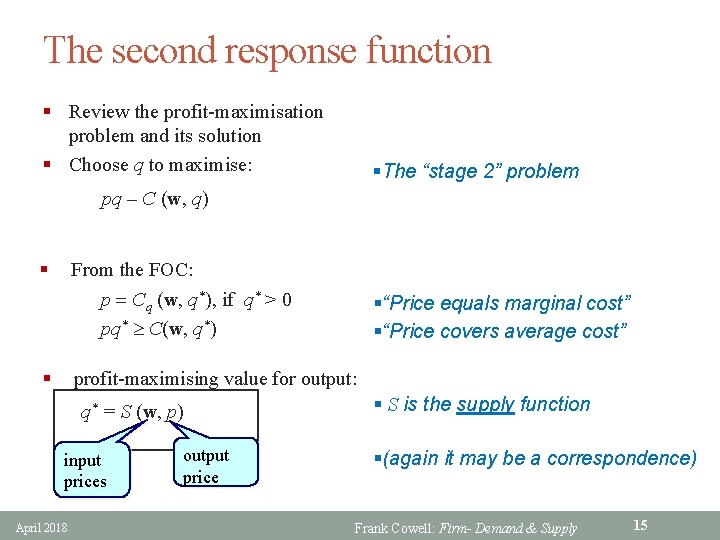
The second response function § Review the profit-maximisation problem and its solution § Choose q to maximise: §The “stage 2” problem pq – C (w, q) § From the FOC: p = Cq (w, q*), if q* > 0 pq* ³ C(w, q*) § §“Price equals marginal cost” §“Price covers average cost” profit-maximising value for output: q* = S (w, p) input prices April 2018 output price § S is the supply function §(again it may be a correspondence) Frank Cowell: Firm- Demand & Supply 15

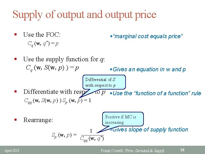
Supply of output and output price § Use the FOC: §“marginal cost equals price” Cq (w, q*) = p § Use the supply function for q: Cq (w, S(w, p) ) = p §Gives an equation in w and p Differential of S with respect to p § Differentiate with respect to p §Use the “function of a function” rule Cqq (w, S(w, p) ) Sp (w, p) = 1 Positive if MC is increasing § Rearrange: 1 Sp (w, p) = ———— Cqq (w, q*) April 2018 §Gives slope of supply function Frank Cowell: Firm- Demand & Supply 16

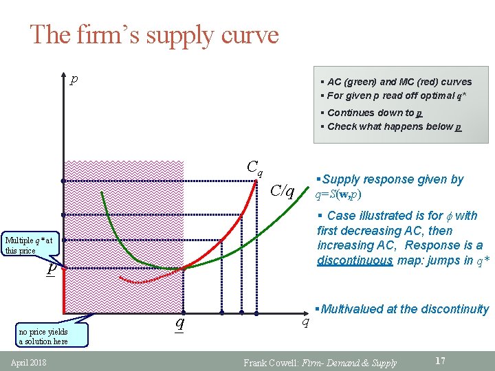
The firm’s supply curve p § AC (green) and MC (red) curves § For given p read off optimal q* § Continues down to p § Check what happens below p Cq §Supply response given by q=S(w, p) C/q § Case illustrated is for f with first decreasing AC, then increasing AC, Response is a discontinuous map: jumps in q* Multiple q* at this price _p – | no price yields a solution here April 2018 _q q §Multivalued at the discontinuity Frank Cowell: Firm- Demand & Supply 17

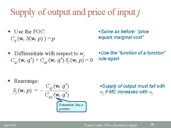
Supply of output and price of input j § Use the FOC: Cq (w, S(w, p) ) = p §Same as before: “price equals marginal cost” §Use the “function of a function” § Differentiate with respect to wj Cqj (w, q*) + Cqq (w, q*) Sj (w, p) = 0 rule again § Rearrange: Cqj (w, q*) Sj (w, p) = – ———— Cqq (w, q*) §Supply of output must fall with wj if MC increases with wj Remember, this is positive April 2018 Frank Cowell: Firm- Demand & Supply 18

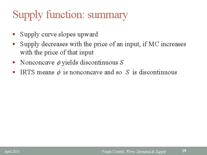
Supply function: summary § Supply curve slopes upward § Supply decreases with the price of an input, if MC increases with the price of that input § Nonconcave f yields discontinuous S § IRTS means f is nonconcave and so S is discontinuous April 2018 Frank Cowell: Firm- Demand & Supply 19

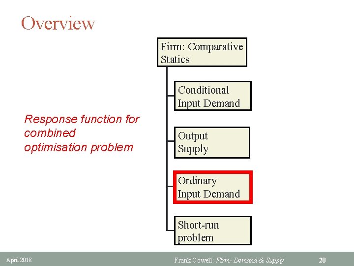
Overview Firm: Comparative Statics Conditional Input Demand Response function for combined optimisation problem Output Supply Ordinary Input Demand Short-run problem April 2018 Frank Cowell: Firm- Demand & Supply 20

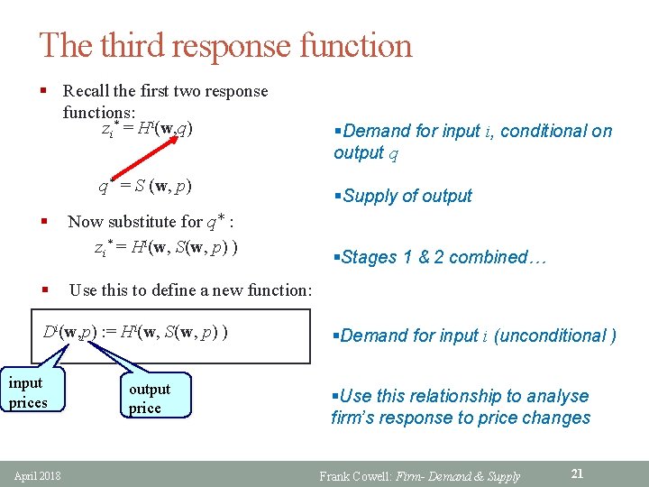
The third response function § Recall the first two response functions: zi* = Hi(w, q) q* = S (w, p) § § Now substitute for q* : zi* = Hi(w, S(w, p) ) April 2018 §Supply of output §Stages 1 & 2 combined… Use this to define a new function: Di(w, p) : = Hi(w, S(w, p) ) input prices §Demand for input i, conditional on output q output price §Demand for input i (unconditional ) §Use this relationship to analyse firm’s response to price changes Frank Cowell: Firm- Demand & Supply 21

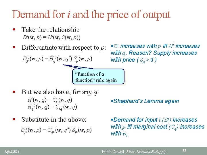
Demand for i and the price of output § Take the relationship Di(w, p) = Hi(w, S(w, p)) § Differentiate with respect to p: §Di increases with p iff Hi increases Dpi(w, p) = Hqi(w, q*) Sp(w, p) with q. Reason? Supply increases with price ( Sp > 0 ) “function of a function” rule again § But we also have, for any q: Hi(w, q) = Ci (w, q) Hqi (w, q) = Ciq (w, q) § Substitute in the above: Dpi(w, p) = Cqi (w, q*) Sp (w, p) April 2018 §Shephard’s Lemma again §Demand for input i (Di) increases with p iff marginal cost (Cq) increases with wi Frank Cowell: Firm- Demand & Supply 22

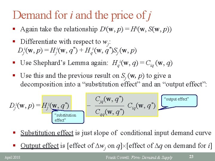
Demand for i and the price of j § Again take the relationship Di(w, p) = Hi(w, S(w, p)) § Differentiate with respect to wj: Dji(w, p) = Hji(w, q*) + Hqi(w, q*)Sj (w, p) § Use Shephard’s Lemma again: Hqi(w, q) = Ciq (w, q) § Use this and the previous result on Sj (w, p) to give a decomposition into a “substitution effect” and an “output effect”: Dji(w, p) = Hji(w, q*) “substitution effect” Cjq(w, q*) Ciq(w, q*) Cqq(w, q*) “output effect” . § Substitution effect is just slope of conditional input demand curve § Output effect is [effect of Dwj on q] [effect of Dq on demand for i] April 2018 Frank Cowell: Firm- Demand & Supply 23

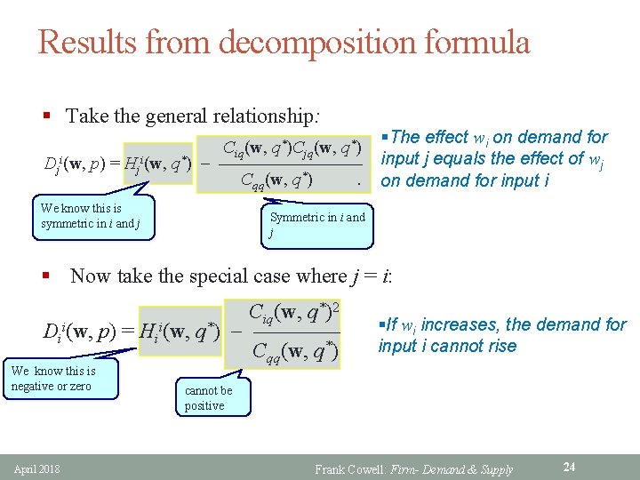
Results from decomposition formula § Take the general relationship: Ciq(w, q*)Cjq(w, q*) Dji(w, p) = Hji(w, q*) Cqq(w, q*). We know this is symmetric in i and j §The effect wi on demand for input j equals the effect of wj on demand for input i Symmetric in i and j § Now take the special case where j = i: Ciq(w, q*)2 Dii(w, p) = Hii(w, q*) Cqq(w, q*). We know this is negative or zero April 2018 §If wi increases, the demand for input i cannot rise cannot be positive Frank Cowell: Firm- Demand & Supply 24

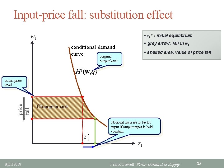
Input-price fall: substitution effect w 1 § z 1* : initial equilibrium § grey arrow: fall in w 1 conditional demand curve original § shaded area: value of price fall output level H 1(w, q) price fall initial price level Change in cost z 1* April 2018 Notional increase in factor input if output target is held constant z 1 Frank Cowell: Firm- Demand & Supply 25

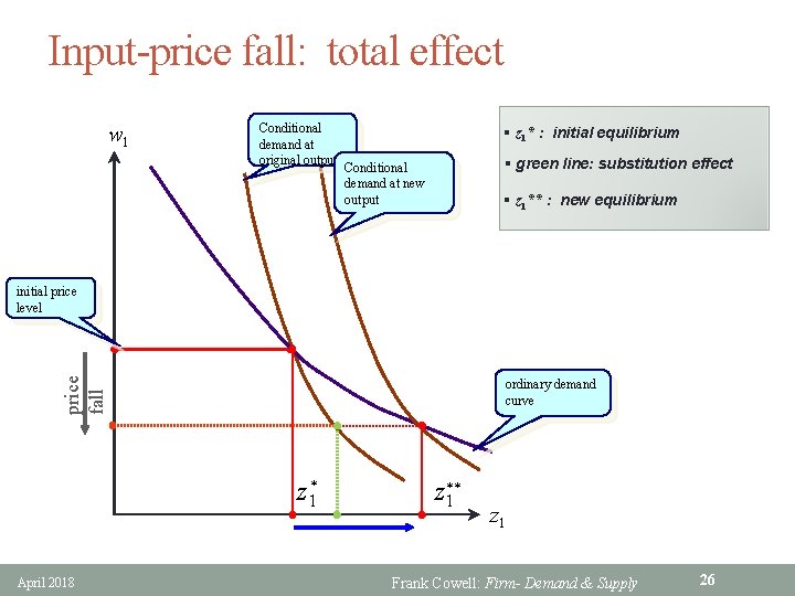
Input-price fall: total effect w 1 Conditional demand at original output § z 1* : initial equilibrium § green line: substitution effect Conditional demand at new output § z 1** : new equilibrium price fall initial price level ordinary demand curve z 1* April 2018 z** 1 z 1 Frank Cowell: Firm- Demand & Supply 26

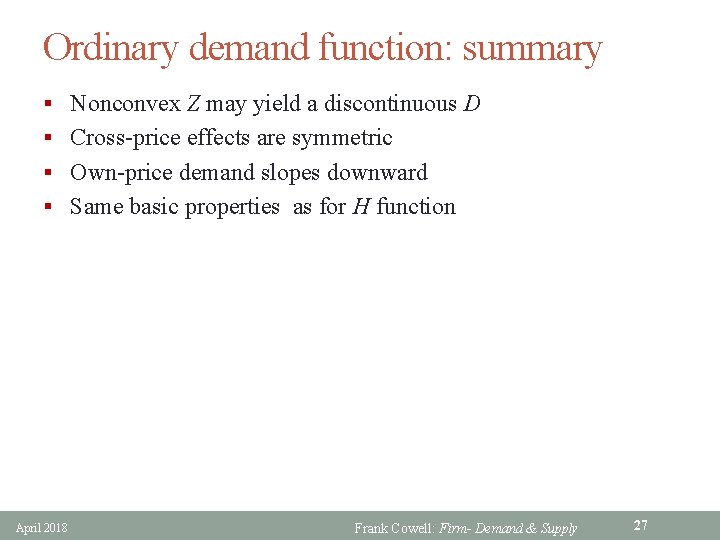
Ordinary demand function: summary § Nonconvex Z may yield a discontinuous D § Cross-price effects are symmetric § Own-price demand slopes downward § Same basic properties as for H function April 2018 Frank Cowell: Firm- Demand & Supply 27

Overview Firm: Comparative Statics Conditional Input Demand Optimisation subject to side-constraint Output Supply Ordinary Input Demand Short-run problem April 2018 Frank Cowell: Firm- Demand & Supply 28

The short run: concept § This is not a moment in time § It is defined by additional constraints within the model § Counterparts in other economic applications where one may need to introduce side constraints April 2018 Frank Cowell: Firm- Demand & Supply 29

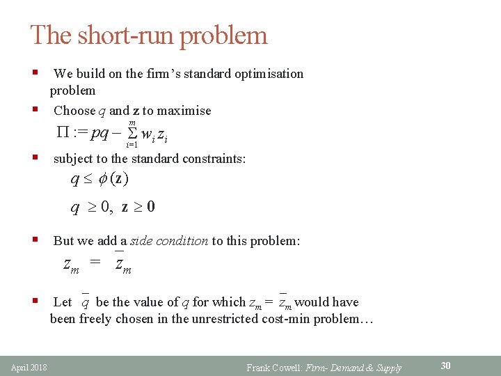
The short-run problem § We build on the firm’s standard optimisation § problem Choose q and z to maximise m P : = pq – S wi zi i=1 § subject to the standard constraints: q f (z) q ³ 0, z ³ 0 § But we add a side condition to this problem: zm = `zm § Let `q be the value of q for which zm =`zm would have been freely chosen in the unrestricted cost-min problem… April 2018 Frank Cowell: Firm- Demand & Supply 30

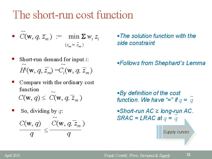
The short-run cost function ~ _ § C(w, q, zm ) : = min S wi zi {zm =`zm } § Short-run demand for input i: ~ _ i H (w, q, zm) =Ci(w, q, zm ) § Compare with the ordinary cost function ~ _ C(w, q) C(w, q, zm ) § So, dividing by q: ~ _ C(w, q) _____ C(w, q, zm ) ______ q q April 2018 §The solution function with the side constraint §Follows from Shephard’s Lemma §By definition of the cost function. We have “=” if q =`q §Short-run AC ≥ long-run AC. SRAC = LRAC at q =`q Supply curves Frank Cowell: Firm- Demand & Supply 31

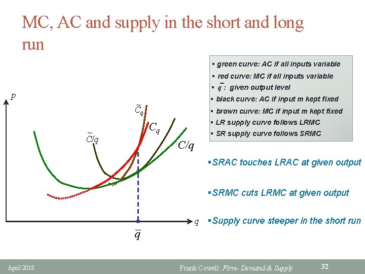
MC, AC and supply in the short and long run § green curve: AC if all inputs variable § red curve: MC if all inputs variable §`q : given output level p § black curve: AC if input m kept fixed ~ Cq § brown curve: MC if input m kept fixed § LR supply curve follows LRMC Cq ~ C/q § SR supply curve follows SRMC C/q §SRAC touches LRAC at given output §SRMC cuts LRMC at given output q April 2018 q §Supply curve steeper in the short run Frank Cowell: Firm- Demand & Supply 32

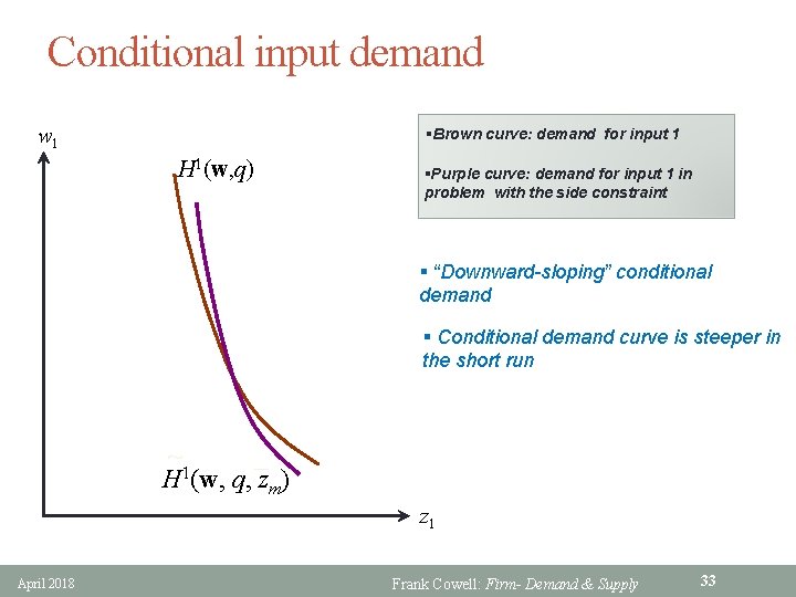
Conditional input demand w 1 §Brown curve: demand for input 1 H 1(w, q) §Purple curve: demand for input 1 in problem with the side constraint § “Downward-sloping” conditional demand § Conditional demand curve is steeper in the short run ~ _ H 1(w, q, zm) z 1 April 2018 Frank Cowell: Firm- Demand & Supply 33

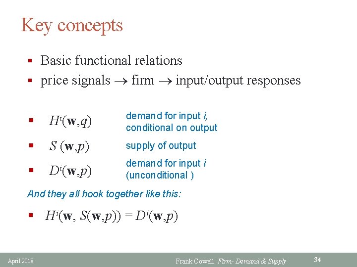
Key concepts § Basic functional relations § price signals firm input/output responses § Hi(w, q) demand for input i, conditional on output § S (w, p) supply of output § Di(w, p) demand for input i (unconditional ) And they all hook together like this: § Hi(w, S(w, p)) = Di(w, p) April 2018 Frank Cowell: Firm- Demand & Supply 34

What next? § Analyse the firm under a variety of market conditions § Apply the analysis to the consumer’s optimisation problem April 2018 Frank Cowell: Firm- Demand & Supply 35