Prerequisites Almost essential Consumer Optimisation CONSUMER WELFARE MICROECONOMICS

Prerequisites Almost essential Consumer Optimisation CONSUMER: WELFARE MICROECONOMICS Principles and Analysis Frank Cowell April 2018 Frank Cowell: Consumer Welfare 1

Using consumer theory Consumer analysis is not just a matter of consumers' reactions to prices § Examine effects of budget changes on consumer's welfare § • changes in incomes • changes in prices § Useful in the design of economic policy • tax structure • subsidies § We can use tools that have become standard in applied microeconomics • price indices • cost-benefit analysis April 2018 Frank Cowell: Consumer Welfare 2

Overview Consumer welfare Utility and income Interpreting the outcome of the optimisation problem in welfare terms CV and EV Consumer’s surplus April 2018 Frank Cowell: Consumer Welfare 3

How to measure a person's “welfare”? We can re-use some concepts § Assume that people know what's best for them § • preferences revealed through behaviour • preference map can be used as a guide to welfare § Re-examine the concept of “maximised utility” • use the indirect utility function • use the cost (expenditure) function April 2018 Frank Cowell: Consumer Welfare 4

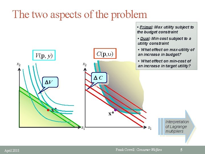
The two aspects of the problem § Primal: Max utility subject to the budget constraint § Dual: Min cost subject to a utility constraint C(p, u) V(p, y) x 2 § What effect on min-cost of an increase in target utility? x 2 C V l x* x 1 April 2018 § What effect on max-utility of an increase in budget? x 1 Frank Cowell: Consumer Welfare Interpretation of Lagrange multipliers 5

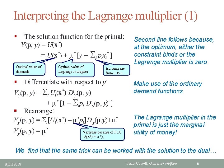
Interpreting the Lagrange multiplier (1) § The solution function for the primal: V(p, y) = U(x*) + m* [y – Optimal value of demands Optimal value of Lagrange multiplier Si pixi* ] Second line follows because, at the optimum, either the constraint binds or the Lagrange multiplier is zero All sums are from 1 to n § Differentiate with respect to y: Vy(p, y) = Si Ui(x*) Diy(p, y) Make use of the ordinary demand functions Vy(p, y) = m* The Lagrange multiplier in the primal is just the marginal utility of money! + m* [1 – Sipi Diy(p, y) ] § Rearrange: Vy(p, y) = Si[Ui(x*) – m*pi]Diy(p, y)+m* Vanishes because of FOC Ui(x*) = m *pi We find that the same trick can be worked with the solution to the dual… April 2018 Frank Cowell: Consumer Welfare 6

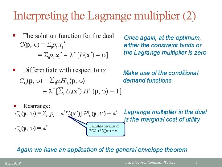
Interpreting the Lagrange multiplier (2) § The solution function for the dual: C(p, u) = Sipi xi* – l* [U(x*) – u] § Differentiate with respect to u: Cu(p, u) = Sipi. Hiu(p, u) Once again, at the optimum, either the constraint binds or the Lagrange multiplier is zero Make use of the conditional demand functions – l* [Si Ui(x*) Hiu(p, u) – 1] § Rearrange: Cu(p, u) = Si [pi – l*Ui(x*)] Hiu(p, u) + l* Cu(p, u) = l* Lagrange multiplier in the dual is the marginal cost of utility Vanishes because of FOC l*Ui(x*) = pi Again we have an application of the general envelope theorem April 2018 Frank Cowell: Consumer Welfare 7

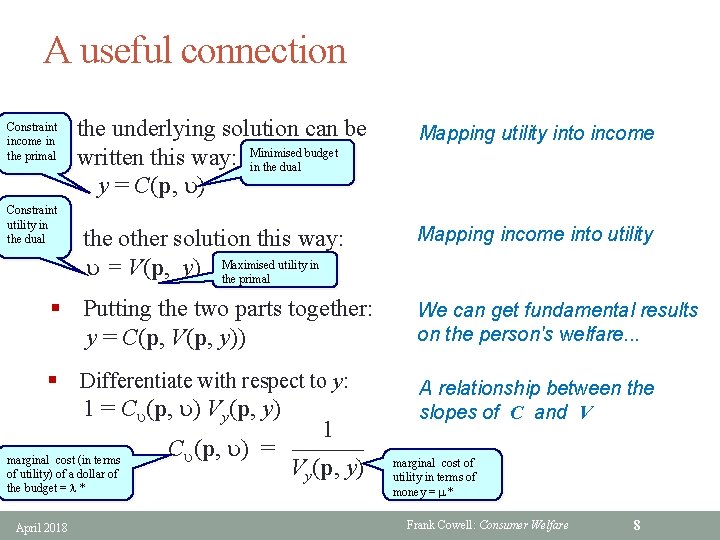
A useful connection § the underlying solution can be budget written this way: Minimised in the dual y = C(p, u) Constraint income in the primal Constraint utility in the dual Mapping utility into income § the other solution this way: utility in u = V(p, y) Maximised the primal Mapping income into utility § Putting the two parts together: y = C(p, V(p, y)) We can get fundamental results on the person's welfare. . . § Differentiate with respect to y: 1 = Cu(p, u) Vy(p, y) 1. Cu(p, u) = ——— marginal cost (in terms Vy(p, y) of utility) of a dollar of the budget = l * April 2018 A relationship between the slopes of C and V marginal cost of utility in terms of money = m * Frank Cowell: Consumer Welfare 8

Utility and income: summary § This gives us a framework for welfare evaluations: • impact of marginal changes of income • interpretation of the Lagrange multipliers § The Lagrange multiplier: • for primal problem is the marginal utility of income • for dual problem is the marginal cost of utility § But does this give us all we need? April 2018 Frank Cowell: Consumer Welfare 9

Utility and income: limitations § This gives us some useful insights but is limited: 1. We have focused only on marginal effects • infinitesimal income changes 2. We have dealt only with income • not the effect of changes in prices § We need a general method of characterising impact of budget changes: • valid for arbitrary price changes • easily interpretable § For the essence of the problem re-examine the basic diagram April 2018 Frank Cowell: Consumer Welfare 10

Overview Consumer welfare Utility and income Exact money measures of welfare CV and EV Consumer’s surplus April 2018 Frank Cowell: Consumer Welfare 11

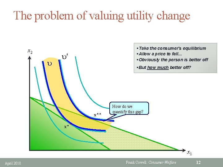
The problem of valuing utility change x 2 u §Take the consumer's equilibrium §Allow a price to fall. . . §Obviously the person is better off u' §But how much better off? x** How do we quantify this gap? x 1 April 2018 Frank Cowell: Consumer Welfare 12

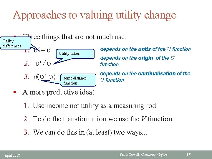
Approaches to valuing utility change § Three things that are not much use: Utility differences 1. u' – u Utility ratios 2. u' / u 3. d(u', u) some distance function depends on the units of the U function depends on the origin of the U function depends on the cardinalisation of the U function § A more productive idea: 1. Use income not utility as a measuring rod 2. To do the transformation we use the V function 3. We can do this in (at least) two ways. . . April 2018 Frank Cowell: Consumer Welfare 13

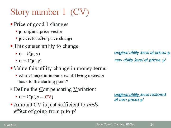
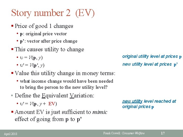
Story number 1 (CV) § Price of good 1 changes • p: original price vector • p': vector after price change § This causes utility to change original utility level at prices p • u = V(p, y) • u' = V(p', y) new utility level at prices p' § Value this utility change in money terms: • what change in income would bring a person back to the starting point? • Define the Compensating Variation: • u = V(p', y – CV) § Amount CV is just sufficient to undo effect of going from p to p' April 2018 original utility level restored at new prices p' Frank Cowell: Consumer Welfare 14

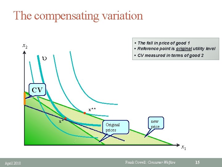
The compensating variation § The fall in price of good 1 § Reference point is original utility level § CV measured in terms of good 2 x 2 u CV x* x** Original prices new price x 1 April 2018 Frank Cowell: Consumer Welfare 15

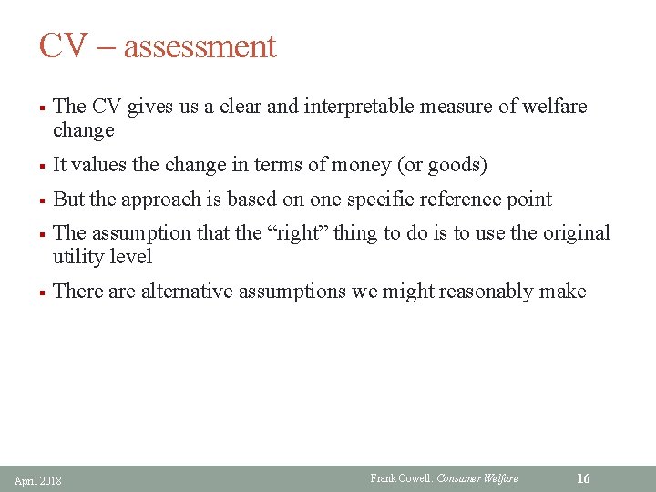
CV assessment § The CV gives us a clear and interpretable measure of welfare change § It values the change in terms of money (or goods) § But the approach is based on one specific reference point § The assumption that the “right” thing to do is to use the original utility level § There alternative assumptions we might reasonably make April 2018 Frank Cowell: Consumer Welfare 16

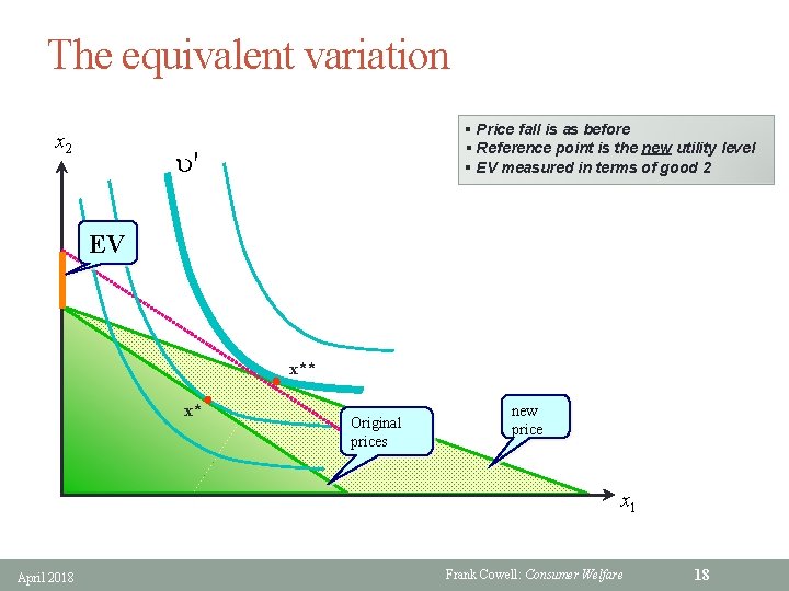
Story number 2 (EV) § Price of good 1 changes • p: original price vector • p': vector after price change § This causes utility to change original utility level at prices p • u = V(p, y) • u' = V(p', y) new utility level at prices p' § Value this utility change in money terms: • what income change would have been needed to bring the person to the new utility level? • Define the Equivalent Variation: • u' = V(p, y + EV) § Amount EV is just sufficient to mimic effect of going from p to p' April 2018 new utility level reached at original prices p Frank Cowell: Consumer Welfare 17

The equivalent variation x 2 § Price fall is as before § Reference point is the new utility level § EV measured in terms of good 2 u' EV x* x** Original prices new price x 1 April 2018 Frank Cowell: Consumer Welfare 18

CV and EV § Both definitions have used the indirect utility function • But this may not be the most intuitive approach • So look for another standard tool As we have seen there is a close relationship between the functions V and C § So we can reinterpret CV and EV using C § • consumer’s cost (or expenditure) function • gives a result measured in monetary terms § The result will be a welfare measure • the change in cost of hitting a welfare level remember: cost decreases mean welfare increases. April 2018 Frank Cowell: Consumer Welfare 19

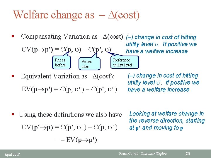
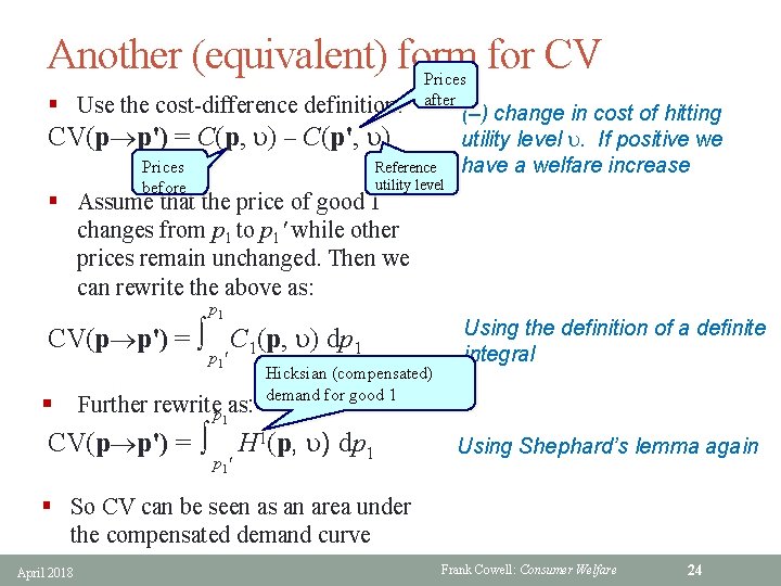
Welfare change as – D(cost) § Compensating Variation as –D(cost): (–) change in cost of hitting utility level u. If positive we have a welfare increase CV(p®p') = C(p, u) – C(p', u) Prices before Prices after Reference utility level § Equivalent Variation as –D(cost): (–) change in cost of hitting utility level u'. If positive we have a welfare increase EV(p®p') = C(p, u' ) – C(p', u' ) § Using these definitions we also have CV(p'®p) = C(p', u' ) – C(p, u' ) Looking at welfare change in the reverse direction, starting at p' and moving to p = – EV(p®p') April 2018 Frank Cowell: Consumer Welfare 20

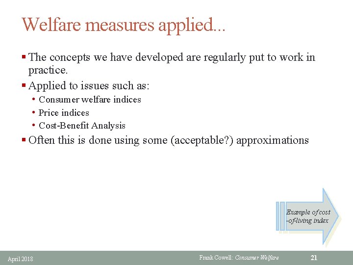
Welfare measures applied. . . § The concepts we have developed are regularly put to work in practice. § Applied to issues such as: • Consumer welfare indices • Price indices • Cost-Benefit Analysis § Often this is done using some (acceptable? ) approximations Example of cost -of-living index April 2018 Frank Cowell: Consumer Welfare 21

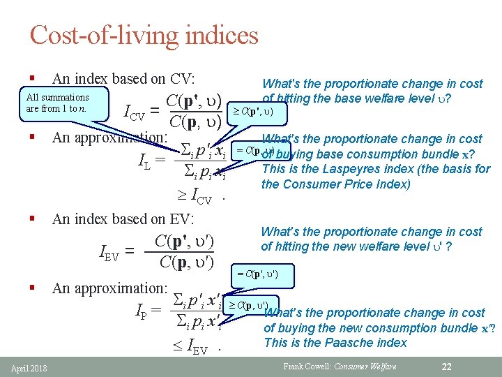
Cost-of-living indices § An index based on CV: All summations are from 1 to n. § C(p', u) ICV = ——— C(p, u) An approximation: IL = What's the proportionate change in cost of hitting the base welfare level u? ³ C(p', u) What's the proportionate change in cost Si p'i xi = C(p, ofu) buying base consumption bundle x? ——— This is the Laspeyres index (the basis for S i pi x i the Consumer Price Index) ³ ICV. § An index based on EV: C(p', u') IEV = ———— C(p, u') § April 2018 What's the proportionate change in cost of hitting the new welfare level u' ? = C(p', u') An approximation: Si p'i x'i IP = ——— Si pi x'i £ IEV. ³ C(p, u') What's the proportionate change in cost of buying the new consumption bundle x'? This is the Paasche index Frank Cowell: Consumer Welfare 22

Overview Consumer welfare Utility and income A simple, practical approach? CV and EV Consumer’s surplus April 2018 Frank Cowell: Consumer Welfare 23

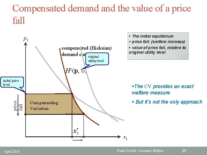
Another (equivalent) form for CV § Use the cost-difference definition: CV(p®p') = C(p, u) – C(p', u) Prices before Prices after Reference utility level (–) change in cost of hitting utility level u. If positive we have a welfare increase § Assume that the price of good 1 changes from p 1 to p 1' while other prices remain unchanged. Then we can rewrite the above as: p 1 CV(p®p') = ò C 1(p, u) dp 1 p 1' Hicksian (compensated) demand for good 1 § Further rewritep 1 as: CV(p®p') = ò H 1(p, u) dp 1 p 1' Using the definition of a definite integral Using Shephard’s lemma again § So CV can be seen as an area under the compensated demand curve April 2018 Frank Cowell: Consumer Welfare 24

Compensated demand the value of a price fall § The initial equilibrium § price fall: (welfare increase) § value of price fall, relative to original utility level p 1 compensated (Hicksian) demand curveoriginal utility level H 1(p, u) price fall initial price level §The CV provides an exact welfare measure § But it’s not the only approach Compensating Variation x*1 April 2018 x 1 Frank Cowell: Consumer Welfare 25

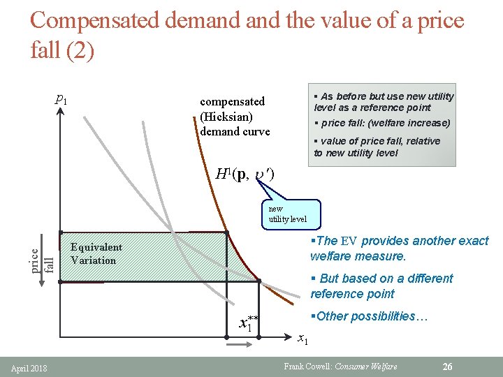
Compensated demand the value of a price fall (2) p 1 § As before but use new utility level as a reference point § price fall: (welfare increase) compensated (Hicksian) demand curve § value of price fall, relative to new utility level H 1(p, u ) price fall new utility level §The EV provides another exact welfare measure. Equivalent Variation § But based on a different reference point x** 1 April 2018 §Other possibilities… x 1 Frank Cowell: Consumer Welfare 26

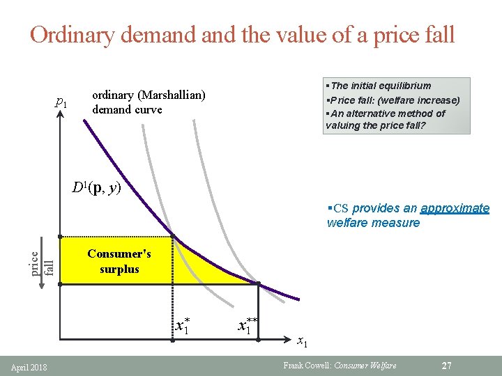
Ordinary demand the value of a price fall p 1 §The initial equilibrium §Price fall: (welfare increase) §An alternative method of valuing the price fall? ordinary (Marshallian) demand curve D 1(p, y) price fall §CS provides an approximate welfare measure Consumer's surplus x*1 April 2018 x** 1 x 1 Frank Cowell: Consumer Welfare 27

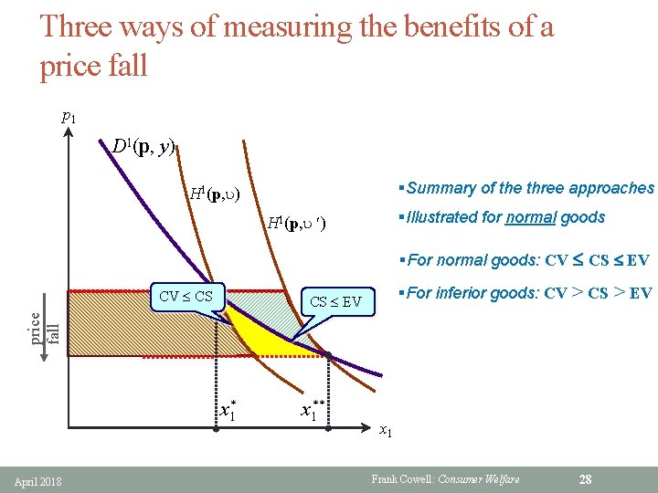
Three ways of measuring the benefits of a price fall p 1 D 1(p, y) §Summary of the three approaches H 1(p, u) §Illustrated for normal goods H 1(p, u ) §For normal goods: CV £ CS £ EV CV £ CS §For inferior goods: CV > CS > EV price fall CS £ EV x 1* April 2018 x 1** x 1 Frank Cowell: Consumer Welfare 28

Summary: key concepts § Interpretation of Lagrange multiplier § Compensating variation § Equivalent variation • CV and EV are measured in monetary units. • In all cases: CV(p®p') = – EV(p'®p) § Consumer’s surplus • The CS is a convenient approximation • For normal goods: CV £ CS £ EV • For inferior goods: CV > CS > EV April 2018 Frank Cowell: Consumer Welfare 29