Preprocessing Chapter 11 What is Preprocessing n Preliminary

Preprocessing Chapter 11

What is Preprocessing n Preliminary image manipulations prior to analysis n Typical operations Radiometric processing to adjust for haze n Geometric processing to register image to map n Cloud masking or land masking n n There is no “standard” set of preprocessing steps

Preprocessing Categories n Three main types n Feature extraction n Radiometric correction n Geometric correction

Feature Extraction n Features are not geographic entities visible on an image n Features refers to statistical characteristics of the data n Individual bands or combinations have information about systematic variation in the scene n In theory, discarded data contain noise and errors n Aim is to improve accuracy of the image

Feature Extraction n Feature extraction can also reduce the number of bands that have to be analyzed Reduces computations n Think about a hyperspectral scanner with over 200 bands n

Feature Extraction n Correlation matrix n Comes from regression analysis

Feature Extraction n The correlation matrix is just the correlations among all possible pairs of bands Correlation Matrix 1 2 3 4 5 6 1 1 2 0. 92 1 3 0. 94 1 4 0. 39 0. 59 0. 48 1 5 0. 49 0. 66 0. 67 0. 82 1 6 0. 03 0. 08 0. 02 0. 18 0. 12 1 7 0. 67 0. 76 0. 82 0. 6 0. 9 0. 02 7 1

Feature Extraction n The correlation matrix is just the correlations among all possible pairs of bands Correlation Matrix 1 2 3 4 5 6 1 1 2 0. 92 1 3 0. 94 1 4 0. 39 0. 59 0. 48 1 5 0. 49 0. 66 0. 67 0. 82 1 6 0. 03 0. 08 0. 02 0. 18 0. 12 1 7 0. 67 0. 76 0. 82 0. 6 0. 9 0. 02 7 1

Feature Extraction n The correlation matrix is just the correlations among all possible pairs of bands Correlation Matrix 1 2 3 4 5 6 1 1 2 0. 92 1 3 0. 94 1 4 0. 39 0. 59 0. 48 1 5 0. 49 0. 66 0. 67 0. 82 1 6 0. 03 0. 08 0. 02 0. 18 0. 12 1 7 0. 67 0. 76 0. 82 0. 6 0. 9 0. 02 7 1

Feature Extraction n The correlation matrix is just the correlations among all possible pairs of bands Correlation Matrix 1 2 3 4 5 6 1 1 2 0. 92 1 3 0. 94 1 4 0. 39 0. 59 0. 48 1 5 0. 49 0. 66 0. 67 0. 82 1 6 0. 03 0. 08 0. 02 0. 18 0. 12 1 7 0. 67 0. 76 0. 82 0. 6 0. 9 0. 02 7 1

Feature Extraction n So bands 3, 5, and 6 carry almost as much information as all seven bands n We could ignore bands 1, 2, 4, and 7 n This is a really simplistic form of feature extraction n Usually more complex and based on statistical relationships

Feature Extraction n Principal Component Analysis (PCA) is such a statistical technique n PCA involves a mathematical procedure that transforms a number of possibly correlated variables into a smaller number of uncorrelated variables called principal components. n The first principal component accounts for as much of the variability in the data as possible, and each succeeding component accounts for as much of the remaining variability as possible.

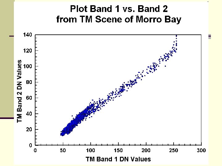
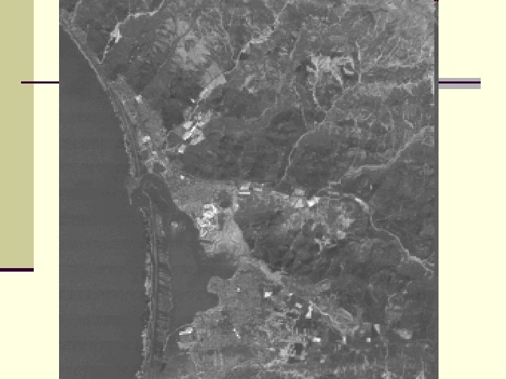
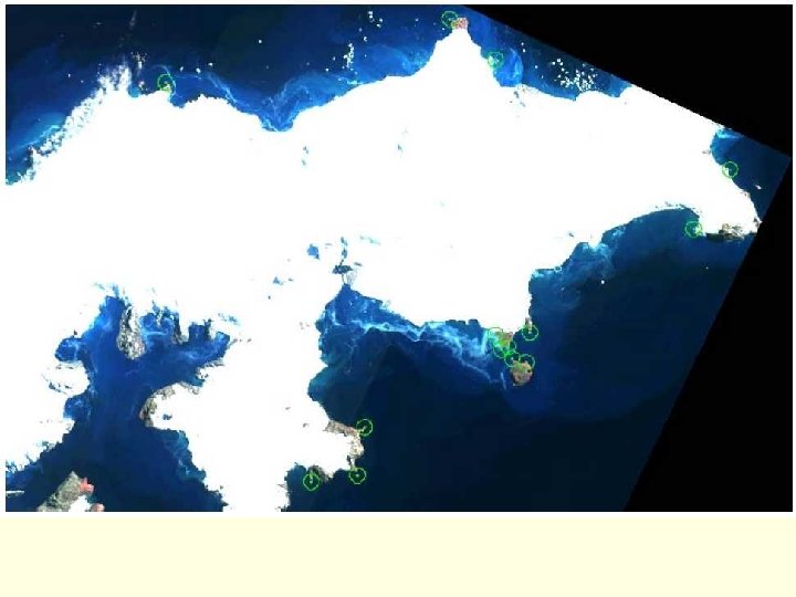
n We’ll use an example from a TM image of Morro Bay, California

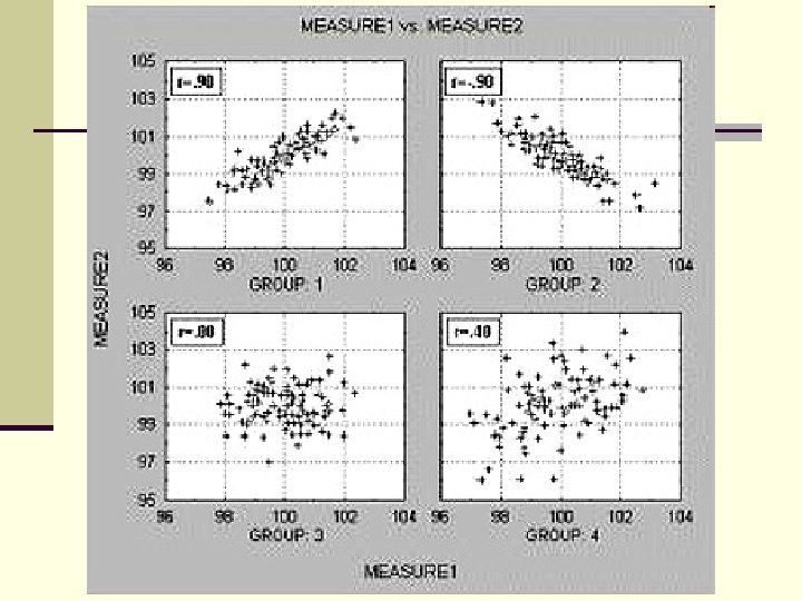
Feature Extraction n This transformation is a rotation of the original axes to new orientations that are orthogonal to each other and therefore there is no correlation between variables. n In the following example there is a high correlation between bands 1 and 2.

New axes Original axes

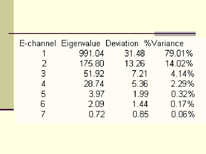
n MSS (Multi-Spectral Scanner) data n For 4 bands PC 1=a. DN 1+ b. DN 2+ c. DN 3+ d. DN 4 n Typically 95% of all variance can be explained by 2 components, so the 'intrinsic dimensionality' of MSS data is 2, n although lower components can display features not visible on bands, otherwise obscured by the main components

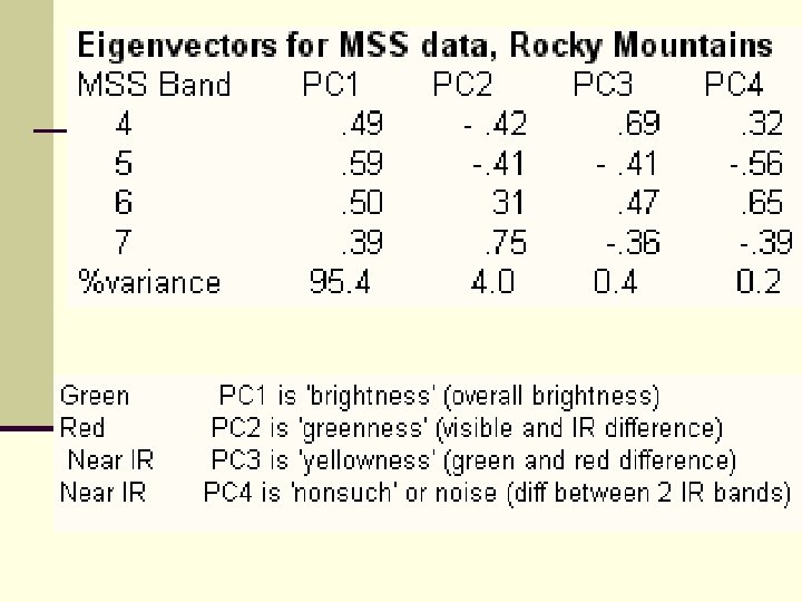
n TM (Thematic Mapper) and ETM data n The seven bands yield up to 7 components, although many users ignore Thermal (band 6) as it is so different. n The components vary according to the scene: forested, mountainous etc. . but generally we see these patterns: n PC 1: 'brightness' the weighted sum of all bands, topography is strong (or cultural data), hydrography weak. . PC 2: 'greenness' (Band 4 v Visible) superior land/water and veg discrimination PC 3: 'Swirness' (Near IR and Visible v Mid (Short. Wave) IR): highlights hydrography and moisture PC 4: Thermal band influence PC 5: Bands 5 v 7 (the two mid IR bands) PC 6: Blue v Red (similar to 1/3 ratio) PC 7: Green v Red (similar to 2/3 ratio)

n Caveats n Since each PC is a linear combination of the original channels one has to be prepared to interpret what they mean n Each image will have its own PC set, which can not be applied to another image n Would have to recalculate for each image

Feature Extraction n PCA determines the optimum linear combination of bands that can account for the variation in pixels n Since the rotation is a linear combination of the original measurements, if all of the axes are included in the rotation, no information is lost. n "No information is lost" means that the original measurements can be recovered from the principal components. n If the original data set is singular, then principal components will produce a new representation that is not singular. n There are several ways of viewing this transformation:

Feature Extraction n It can be viewed as a rotation of the existing axes to new positions in the space defined by the original variables. n In this new rotation, there will be no correlation between the new variables defined by the rotation. n The first new variable contains the maximum amount of variation, the second new variable contains the maximum amount of variation unexplained by the first and orthogonal to the first, etc. . .

Feature Extraction n It can be viewed as finding a projection of the observations onto orthogonal axes contained in the space defined by the original variables. n The criteria being that the first axis "contains" the maximum amount of variation, or "accounts" for the maximum amount of variation. n The second axis contains the maximum amount of variation orthogonal to the first. n The third axis contains the maximum amount of variation orthogonal to the first and second axis and so on until one has the last new axis which is the last amount of variation left.

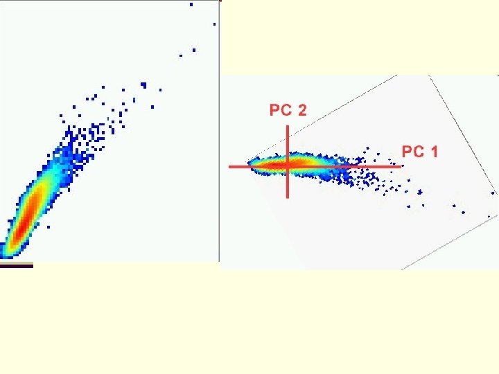
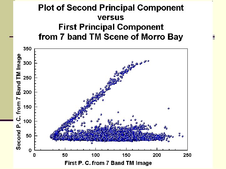
n How do we get this figure? n The elliptical cloud that lies parallel to the X axis is what we might expect. n But, need to remember that this is a rigid rotation of axes in a 7 dimensional space, one for each band (or variable). n We can see here that the original data was not Multivariate Normal, an assumption that would need to be met if one wanted to carry out any parametric statistical tests. n This non-normality is indicated the anomalous cloud of points going diagonally across the graph. If the data were multivariate normal in 7 dimensions, then the plot would only have a cloud like the horizontal one in the above plot.

n Let's check TM bivariate scatter plots for the Morro Bay bands. n Various combinations were tried, but an interesting one is Band 2 (abscissa) vs Band 4 (ordinate):

n This plot shows a bimodal distribution of data points. n The upper (blue & purple dots) plot shows strong correlation (spread around a mean line is small) between the two bands. n This plot is for all the water in the scene - the DNs for water extend over a wide range of values but value changes in one band are matched by similar change increments in the other band. n The second plot (orange/yellow/green) is for all other classes in the image. n n There is strong correlation when DN values are low but as these increase for both bands the plot widens. This means that for much of the DN value range, the two bands are less correlated and should serve increasingly well as discriminators in any classification.

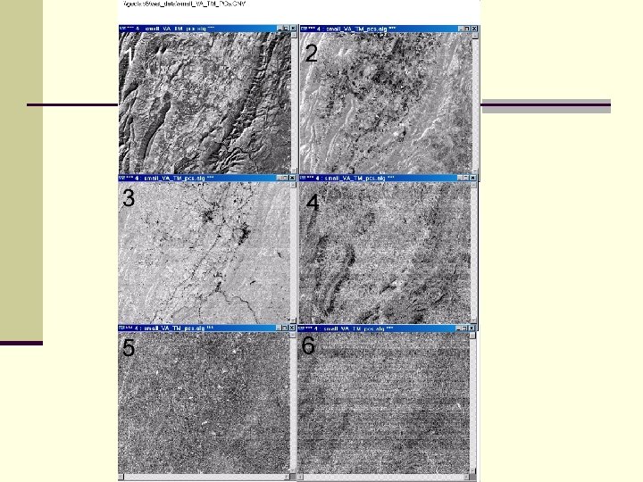
n PCA output is a new set of DN pixels for each derived component. n The DN set can be made to appear as an image that resembles to some extent any of the individual TM bands. n We will now look at each of these components as images, keeping in mind that many of the tonal patterns in individual components do not seem to spatially match specific features or classes identified in the TM bands and represent linear combinations of the original values instead. n We make only limited comments on the nature of those patterns that lend themselves to some interpretation.

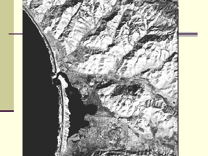
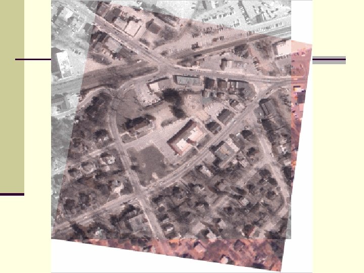
n The first Principal Component contains the maximum amount of variation in the 7 -dimensional space defined by the seven Thematic Mapper bands. n The image produced from PC 1 data commonly resembles an actual aerial photograph. n n n This is normal for the first component, in that it broadly simulates standard black and white photography and it contains most of the pertinent information inherent to a scene. The hills appear more realistic because the sharp lightdark contrast in most TM bands is subdued. Note the internal structure of the waves and the absence of any indication of sediment load in the sea.

n The histogram of PC 1 shows two peaks n The first, on the left, are the ocean pixels and the second one, to the right, the land pixels.

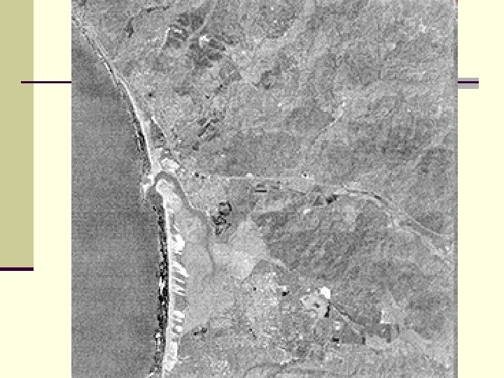
n For PC 2, the bulk of the pixels falls in such a narrow range, the image does not seem to have much interpretable patterns

n PC 2 image histogram equalization stretched n Breaking waves are singled out as very bright

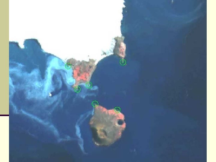
n Some of the gray patterns in the PC 3 image below can be broadly correlated with two combined classes of vegetation: The brighter tones come from the fairways in the golf course and many of the agricultural fields. n Moderately darker tones coincide with some of the grasslands, forest or tree areas, and coastal marshland. n Note that both the beach and waves almost disappear as patterns. n

n The breakers completely disappear in the PC 4 image, while the rest of the scene is rather flat and mostly dark but with several areas of medium grays.

n You may be wondering what the remaining PCs (through PC 7) look like, and if they show any useful information. n The response, after examining, for example, PC 6, is that the features we are familiar with do appear but probably offer little new in interpretation. n Note that the waves in the image below now are black - interesting but perhaps meaningless; the golf course pattern is also black.

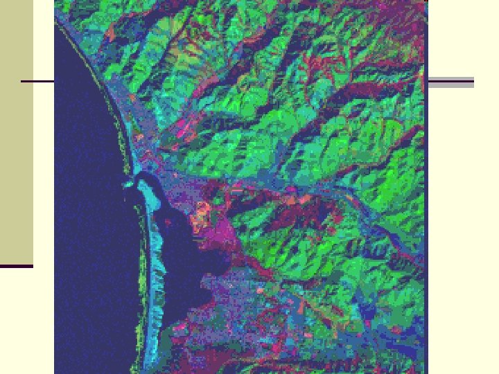
n The information in PCA images can be revealed better by combining them visually as registered overlays. n Any three of these PC images can be made into color composites with various assignments of blue, green, and red. n In all, 24 different combinations are possible.

n The next image composed of PC 4 = blue, PC 1 = n n n green, and PC 3 = red. In this rendition, the golf course has a singular color signature (orange-red) and a unique internal structure. Most other vegetation shows as red to purple-red tones, but the grasslands (v) has an unusual color, describable as greenish-orange. The brighter slopes of the hills and mountains appear as medium green, while some areas in shadow, are bluish. The urban areas also have a deep blue color. The beach bar now appears as turquoise and the adjacent breakers are olive-green.

Subsets n Does not seem to be very challenging n Often have to “register” by matching to another data set n Convenient to prepare subsets before registration due to increased computation with large images But if subset is too small, ther may not be enough Ground Control Points n Have to use an intermediate size subset n

Subsets n Subsets should be large enough to provide context n Enough training sites for accuracy

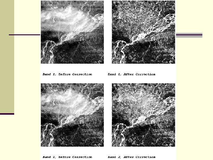
Radiometric Preprocessing n Many operations are image restoration n Help to remove interferences and noise n Brightness of the surface is what is desired n Brightness from atmosphere can contribute to overall brightness

Radiometric Preprocessing n Atmospheric corrections in 3 categories n Model physical behavior of EM radiation through the atmosphere n n Advantages are rigor and wide applicability Disadvantages – very complex, require detailed meteorological information

Radiometric Preprocessing n Examination of reflectances from objects of known brightness n n IR is absorbed by water, so should be black If different, could subtract that value from all the pixels § Known as histogram minimum method (HMM) or the dark object subtraction (DOS) technique.

Radiometric Preprocessing n A more sophisticated alternative is to look at brightness among several bands n A regression technique can be used to to pair individual band values with the value in the NIR The Y intercept is the correction for the particular band n This technique can be applied to localized areas of the scene n

Radiometric Preprocessing n An improvement on the regression technique uses the variance-covariance matrix This is the set of variances and covariances between all the band pairs n This is called the Covariance Matrix Method (CMM) n

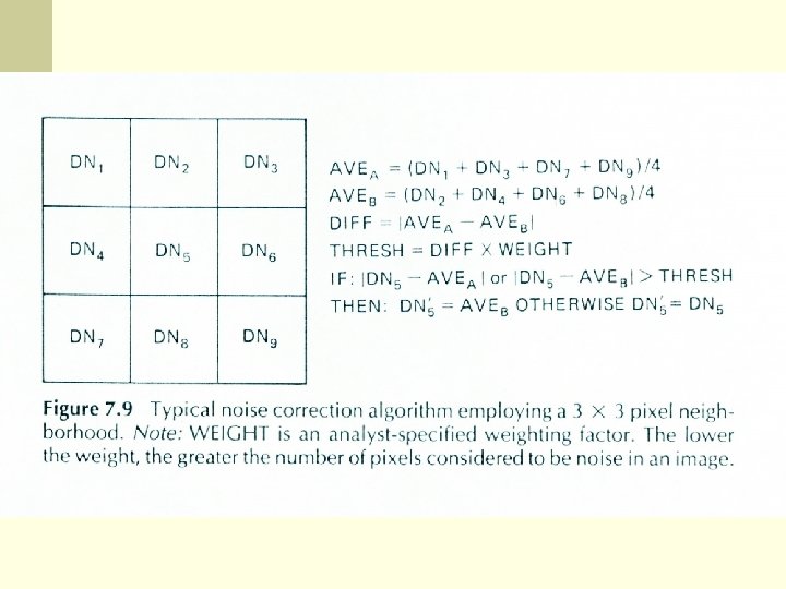
Destriping n The Landsat MSS sometimes show an error known as sixth-line striping Caused by differences in detector sensitivities n Show up as brighter or darker values than adjacent lines n n Overall character is not much affected, but it looks ugly.

Destriping n A number of algorithms have been developed to correct the problem n Each tries to replace the stripe with recalculated values n Two common approaches n Adjacent value replacement n Use mean and standard deviation of bad line, and correct to those of good bands.

Destriping n Filtering may also be a viable option n Asymmetric low pass filter horizontally

Destriping n High-pass vertically and divide original by line detect image

Image Matching n This is superimposing two images on top of each other. n For example in change detection n A common method is to overlay the two images digitally and calculate a correlation for the area of overlap Matched positions are shifted pixel by pixel and a new correlation value is calculated n The optimum is presumed the correct position n The two images are not changed n

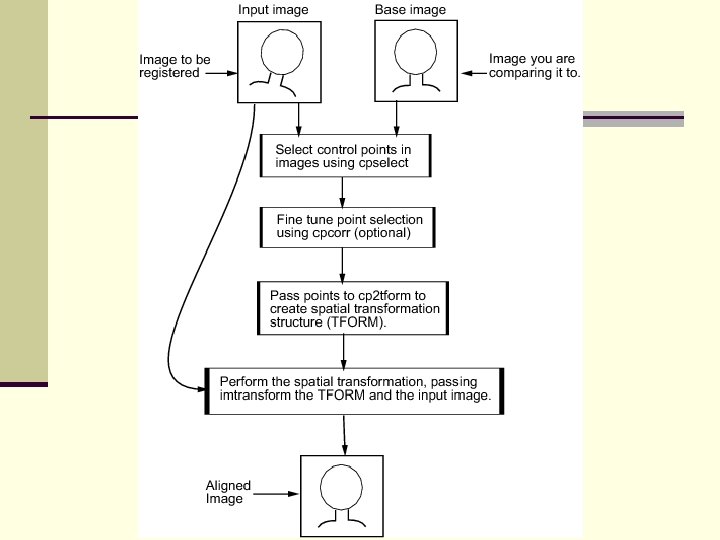
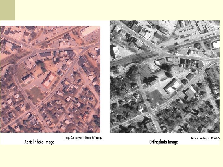
Image Matching n The most common problem is image registration or geometric correction One image is the “correct” version – a base image or “map” n The second is altered to fit the base image. n n A rigorous approach is to use the sensor geometry and motion to calculate pixel coordinates n Requires precise orbital parameters and Earth’s shape

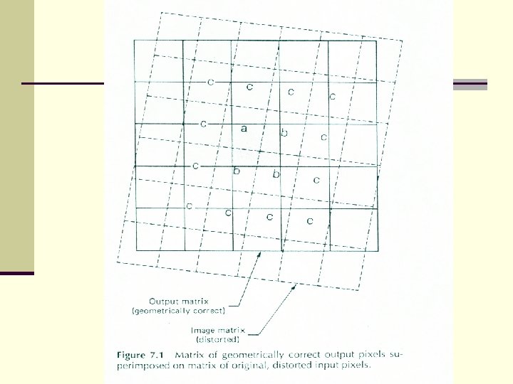
Geometric Correction n Another approach is to simply consider the image as a raster that is manipulated into a different shape.

Geometric Correction n Then the program has to recalculate positions of pixels n This can be done by a number of different methods n The simplest is the value from the nearest uncorrected pixel n n This is called nearest-neighbor resampling However, it can cause positional errors especially visible in linear features

Geometric Correction n Bilinear interpolation is another resampling technique that is based on a weighted average of the four nearest neighbors. Weighted is in terms of how close each of the nearest neighbors is, closer have more weight n Original brightness values are lost n n n Range of the original may differ from resampled image Decreases spatial resolution because of “smearing”

Geometric Correction n Cubic Convolution is the most sophisticated and complex Uses weighted average of sixteen nearest neighbor pixels n Resulting images are most attractive, buit also most altered n Need more GCPs n Computations are more intensive n

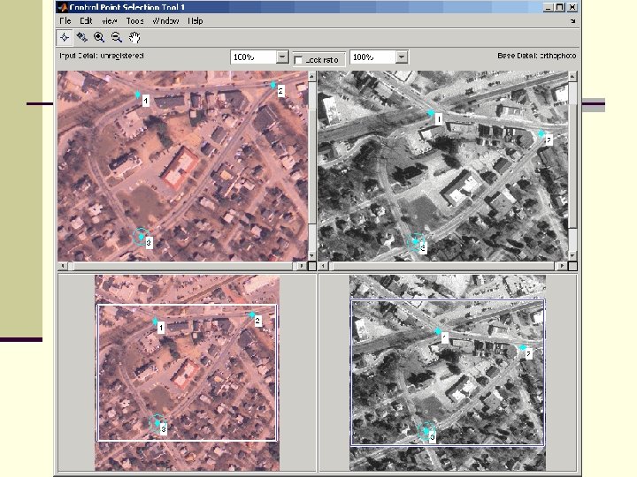
Geometric Correction n Guidelines for identifying GCPs n Need to be able to identify them on both images – intersections are good n Should be dispersed throughout the image, especially near edges n It is better to have more GCPs because the error decreases n n Look at the RMS column in Imagine At least 16 if they can be located with an accuracy of 1/3 rd of a pixel

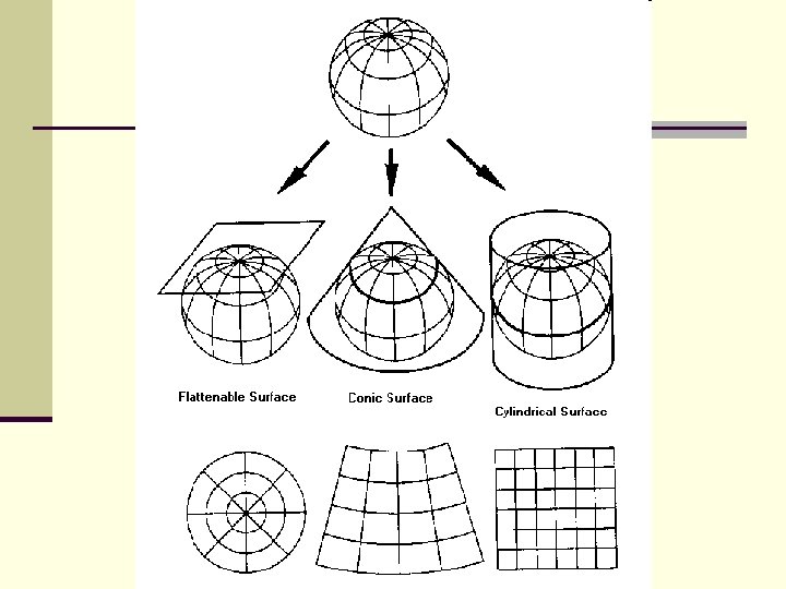
Map Projections n Both the earth and the satellites are moving n This makes mapping difficult with standard map projections n Sun-synchronous orbits described curved paths over the earth’s surface. n Snyder (1981) devised projections that will show satellite tracks as straight lines Used cylindrical projection for global maps n Conic projection for continental maps n

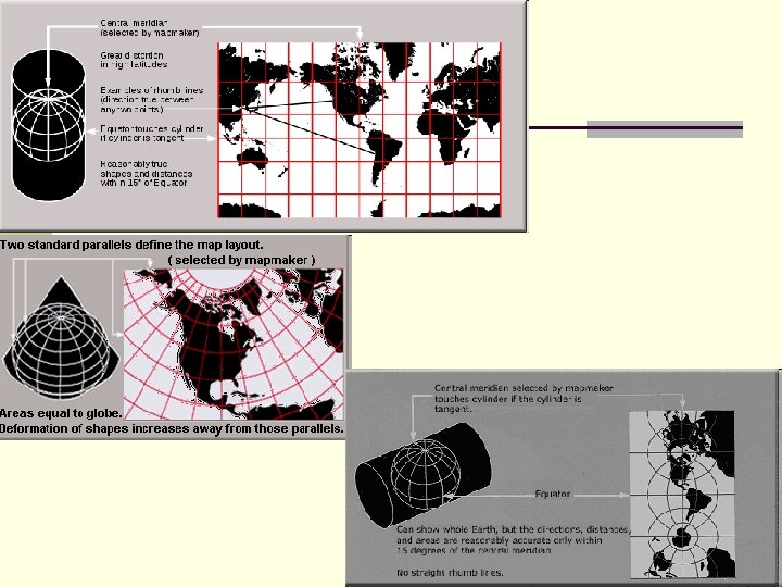
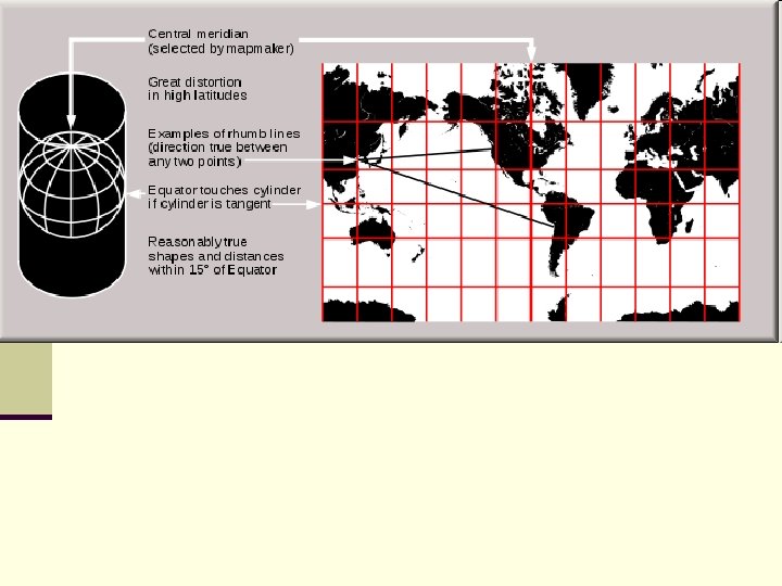
Map Projections n If a Mercator projection is tangent at the equator, it represents the earth exactly as it is there and only there. As you move away from the equator, the distortion becomes greater n Area errors are very large at the poles n Shape is shown accurately n A useful aspect for navigation is that a constant compass bearing is a straight line n

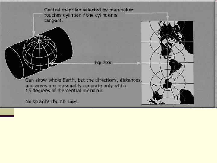
Map Projections n Transverse Mercator is tangent at a meridian (longitude) – so the cylinder is turned sideways. n If you do this for all meridians, and retain only the center strip, you get a very accurate map of the Earth n This is what is done for the Universal Transverse Mercator (UTM) projection

Transverse Mercator projection

Map Projections n Oblique Mercator projections are tangent along a great circle at an angle to the equator other than 90º.

Map Projections n Colvocoresses (1974) developed the Space Oblique Mercator (SOM)projections

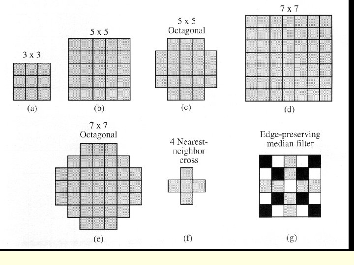
Image Filtering n Noise removal n Smoothing n Edge enhancement n Most image enhancement operations work the same way n A moving window

Filter example n Use a smoothing filter n 1 1 1 n Multiply each element in the raster by 1, sum the results, divide by 9 and replace the central pixel in the original data set 10 20 10 n 10 20 10 = > 10 13 10 10 20 10

Filter example n A sample data set

Filter example n Smoothing filter result

Filter example n Now lets try a linear gradient filter n -1 0 1 n Since the numbers may become negative, a constant is added to the result. n In this case add 100

Filter example n A sample data set again

Filter example n Linear gradient filter result

Filters n Filters can often be used in combination n These three directional filters are orthogonal to each other, and the result is a non-directional filtered product that enhances linear features

The kernel or window n The factors in the moving window are specified based on the desired result n The 3 X 3 array moves across the image and converts the value of the center pixel based on the operations specified by the surrounding pixels

A ‘high pass’ filter or kernel

Directional Edge Enhancement… examples

Effects of Preprocessing n It should be clear that there may be unwanted effects of preprocessing n However, there are few studies that have looked at the effects

Data Fusion n Data fusion refers to incorporating images of different resolutions into a single frame n High res panchromatic with coarse res MSS n These are valuable because they bring different sources of information together n Require that the images were acquired close to the same time

Data Fusion n Processing requires that the images are registered n Spectral domain procedures project the MSS into spectral data space, then create a new band (transformed) that is most closely correlated with the pan image

Data Fusion n Color as we perceive it can be described by intensity – hue – saturation (IHS) Intensity is brightness n Hue is the dominant wavelength (color) n Saturation is the purity of the color (bandwidth) n n So the RGB image is transformed into a IHS space n The high res pan image is stretched to approximate the mean and variance of Intensity

Data Fusion n The stretched pan image is then substituted for the intensity component of the original MSS image n This image is then projected back into RGB space n So the intensity of the high res image which has higher spatial detail is then used in the original image

Data Fusion n Other techniques include the use of Principal Component transformation (PCT) n PCA of low res, then stretched hig res is substituted for PC I and image is reconstructed n Spatial Domain Procedures extract high- frequency variations of the high res image and insert it into the low res image n High pass filter (HPF) technique, the high-pass image is then inserted into the low res

Data Fusion n Algebraic procedures n Tries to assign the correct brightness to the replacement band n Multiplicative model (MLT) multiplies each pixel in MSS by a pixel in the high res image n The important thing here is that fused images are intended for visual interpretation only n Not to be used for digital classification or analysis

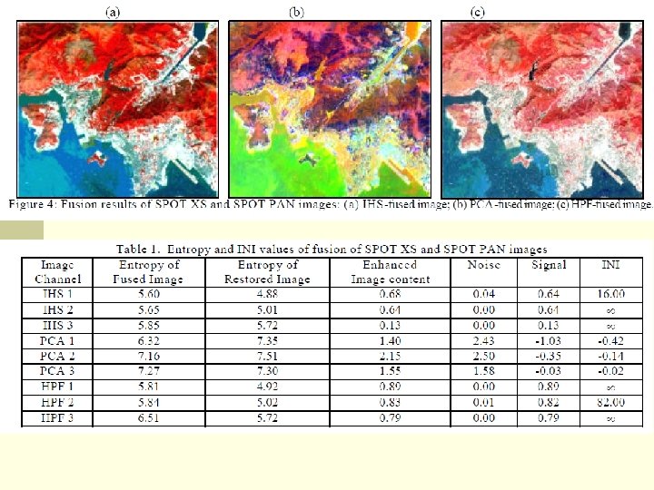
Data Fusion

Data Fusion n The HIS and HPF images produced high INI values = increased information and almost no noise n PCA images had negative values indicating no information content increase, and high noise causing deterioration of the image