Predictive Modeling and Analysis 8 1 LogicDriven Modeling

Predictive Modeling and Analysis 8 -1

�Logic-Driven Modeling �Data-Driven Modeling �Analyzing Uncertainty and Model Assumptions �Model Analysis Using Risk Solver Platform 8 -2

Logic-Driven Modeling �Predictive modeling is the heart and soul of business decisions. �Building decision models is more of an art than a science. �Creating good decision models requires: - solid understanding of business functional areas - knowledge of business practice and research - logical skills �It is best to start simple and enrich models as necessary. Copyright © 2013 Pearson Education, Inc. publishing as Prentice Hall 8 -3

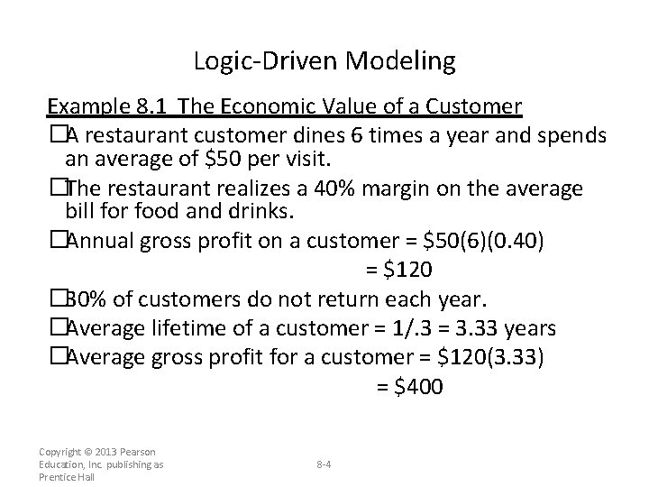
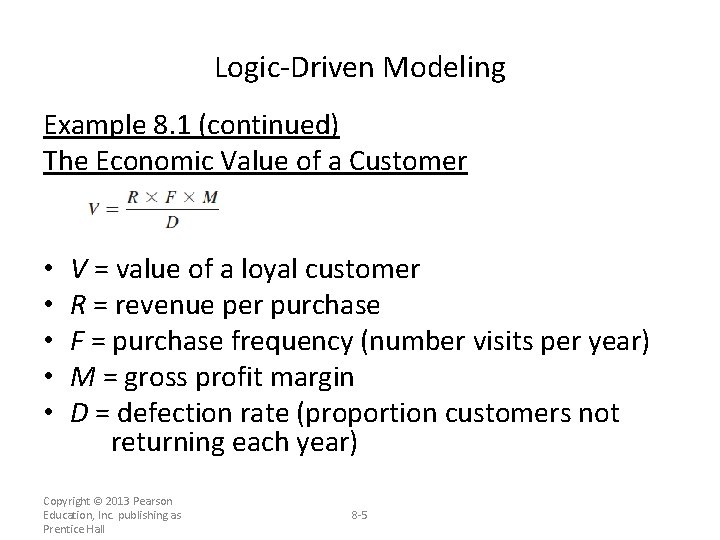
Logic-Driven Modeling Example 8. 1 The Economic Value of a Customer �A restaurant customer dines 6 times a year and spends an average of $50 per visit. �The restaurant realizes a 40% margin on the average bill for food and drinks. �Annual gross profit on a customer = $50(6)(0. 40) = $120 � 30% of customers do not return each year. �Average lifetime of a customer = 1/. 3 = 3. 33 years �Average gross profit for a customer = $120(3. 33) = $400 Copyright © 2013 Pearson Education, Inc. publishing as Prentice Hall 8 -4

Logic-Driven Modeling Example 8. 1 (continued) The Economic Value of a Customer • • • V = value of a loyal customer R = revenue per purchase F = purchase frequency (number visits per year) M = gross profit margin D = defection rate (proportion customers not returning each year) Copyright © 2013 Pearson Education, Inc. publishing as Prentice Hall 8 -5

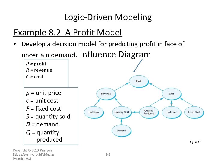
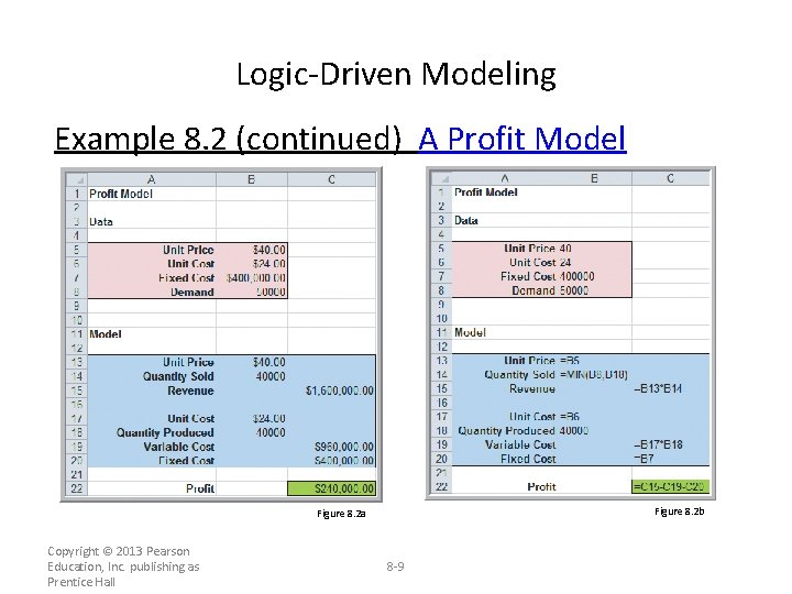
Logic-Driven Modeling Example 8. 2 A Profit Model • Develop a decision model for predicting profit in face of uncertain demand. Influence Diagram P = profit R = revenue C = cost p = unit price c = unit cost F = fixed cost S = quantity sold D = demand Q = quantity produced Copyright © 2013 Pearson Education, Inc. publishing as Prentice Hall Figure 8. 1 8 -6

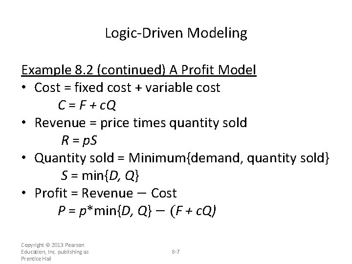
Logic-Driven Modeling Example 8. 2 (continued) A Profit Model • Cost = fixed cost + variable cost C = F + c. Q • Revenue = price times quantity sold R = p. S • Quantity sold = Minimum{demand, quantity sold} S = min{D, Q} • Profit = Revenue − Cost P = p*min{D, Q} − (F + c. Q) Copyright © 2013 Pearson Education, Inc. publishing as Prentice Hall 8 -7

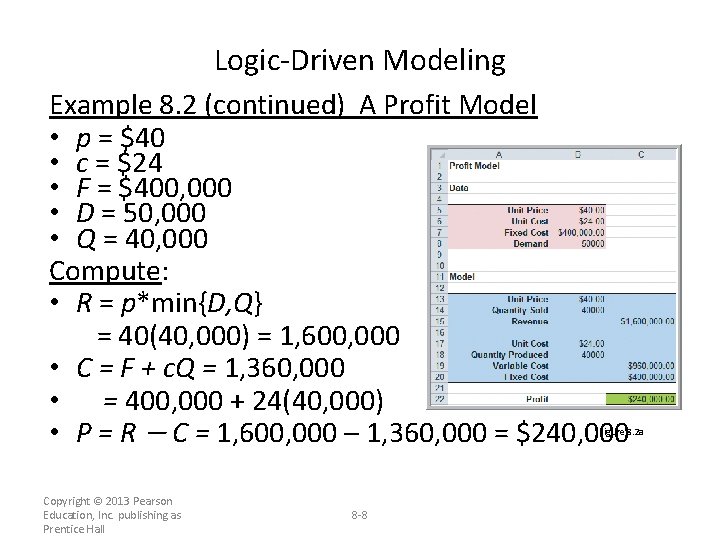
Logic-Driven Modeling Example 8. 2 (continued) A Profit Model • p = $40 • c = $24 • F = $400, 000 • D = 50, 000 • Q = 40, 000 Compute: • R = p*min{D, Q} = 40(40, 000) = 1, 600, 000 • C = F + c. Q = 1, 360, 000 • = 400, 000 + 24(40, 000) • P = R − C = 1, 600, 000 – 1, 360, 000 = $240, 000 Figure 8. 2 a Copyright © 2013 Pearson Education, Inc. publishing as Prentice Hall 8 -8

Logic-Driven Modeling Example 8. 2 (continued) A Profit Model Figure 8. 2 b Figure 8. 2 a Copyright © 2013 Pearson Education, Inc. publishing as Prentice Hall 8 -9

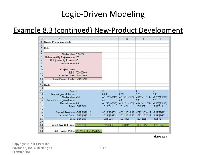
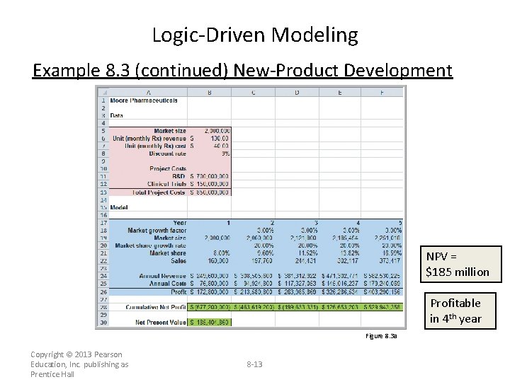
Logic-Driven Modeling Example 8. 3 New-Product Development �Moore Pharmaceuticals needs to decide whether to conduct clinical trials and seek FDA approval for a newly developed drug. Estimated figures: �R&D cost = $700 million �Clinical trials cost = $150 million �Market size = 2 million people �Market size growth = 3% per year Copyright © 2013 Pearson Education, Inc. publishing as Prentice Hall 8 -10

Logic-Driven Modeling Example 8. 3 (continued) New-Product Development Additional estimated figures �Market share = 8% �Market share growth = 20% per year (for 5 years) �Revenue from a monthly prescription = $130 �Variable cost for a monthly prescription = $40 �Discount rate for net present value = 9% Moore Pharmaceuticals wants to determine net present value for the next 5 years and to determine how long it will take to recover fixed costs. Copyright © 2013 Pearson Education, Inc. publishing as Prentice Hall 8 -11

Logic-Driven Modeling Example 8. 3 (continued) New-Product Development Figure 8. 3 b Copyright © 2013 Pearson Education, Inc. publishing as Prentice Hall 8 -12

Logic-Driven Modeling Example 8. 3 (continued) New-Product Development NPV = $185 million Profitable in 4 th year Figure 8. 3 a Copyright © 2013 Pearson Education, Inc. publishing as Prentice Hall 8 -13

Data-Driven Modeling Relationships and Trends in Data • Create charts to better understand data sets. • For cross-sectional data, use a scatter chart. • For time series data, use a line chart. • Consider using mathematical functions to model relationships. Copyright © 2013 Pearson Education, Inc. publishing as Prentice Hall 8 -14

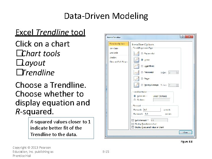
Data-Driven Modeling Excel Trendline tool Click on a chart �Chart tools �Layout �Trendline Choose a Trendline. Choose whether to display equation and R-squared values closer to 1 indicate better fit of the Trendline to the data. Figure 8. 8 Copyright © 2013 Pearson Education, Inc. publishing as Prentice Hall 8 -15

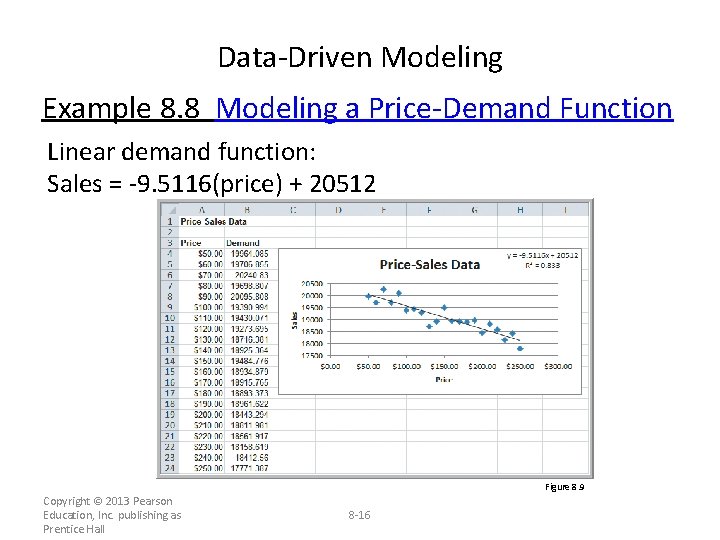
Data-Driven Modeling Example 8. 8 Modeling a Price-Demand Function Linear demand function: Sales = -9. 5116(price) + 20512 Copyright © 2013 Pearson Education, Inc. publishing as Prentice Hall Figure 8. 9 8 -16

Analyzing Uncertainty and Model Assumptions What-If Analysis • Spreadsheet models allow you to easily evaluate what-if questions. • How do changes in model inputs (that reflect key assumptions) affect model outputs? • Systematic approaches to what-if analysis make the process easier and more useful. Copyright © 2013 Pearson Education, Inc. publishing as Prentice Hall 8 -17

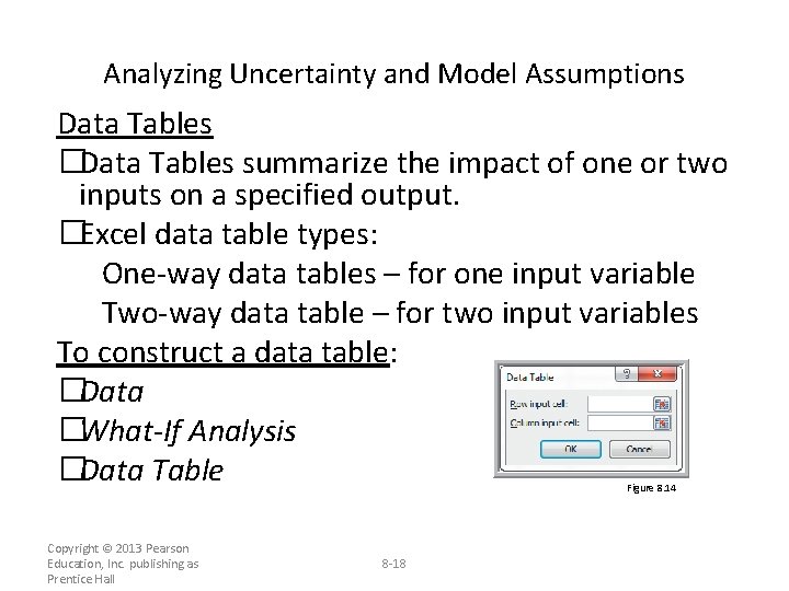
Analyzing Uncertainty and Model Assumptions Data Tables �Data Tables summarize the impact of one or two inputs on a specified output. �Excel data table types: One-way data tables – for one input variable Two-way data table – for two input variables To construct a data table: �Data �What-If Analysis �Data Table Figure 8. 14 Copyright © 2013 Pearson Education, Inc. publishing as Prentice Hall 8 -18

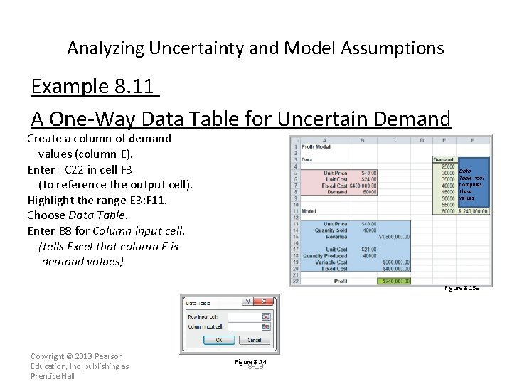
Analyzing Uncertainty and Model Assumptions Example 8. 11 A One-Way Data Table for Uncertain Demand Create a column of demand values (column E). Enter =C 22 in cell F 3 (to reference the output cell). Highlight the range E 3: F 11. Choose Data Table. Enter B 8 for Column input cell. (tells Excel that column E is demand values) Data Table tool computes these values Figure 8. 15 a Copyright © 2013 Pearson Education, Inc. publishing as Prentice Hall Figure 8. 14 8 -19

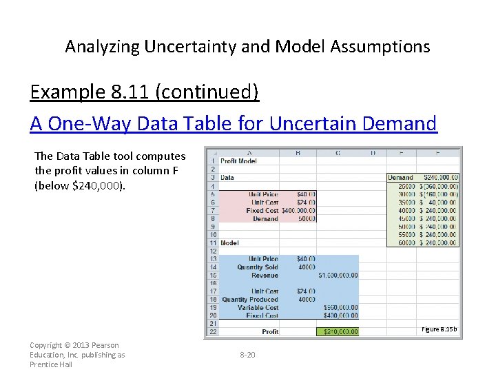
Analyzing Uncertainty and Model Assumptions Example 8. 11 (continued) A One-Way Data Table for Uncertain Demand The Data Table tool computes the profit values in column F (below $240, 000). Figure 8. 15 b Copyright © 2013 Pearson Education, Inc. publishing as Prentice Hall 8 -20

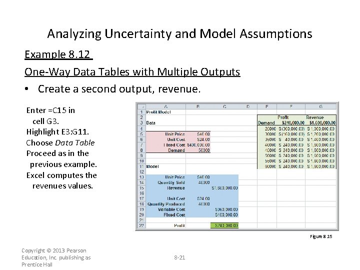
Analyzing Uncertainty and Model Assumptions Example 8. 12 One-Way Data Tables with Multiple Outputs • Create a second output, revenue. Enter =C 15 in cell G 3. Highlight E 3: G 11. Choose Data Table Proceed as in the previous example. Excel computes the revenues values. Figure 8. 15 Copyright © 2013 Pearson Education, Inc. publishing as Prentice Hall 8 -21

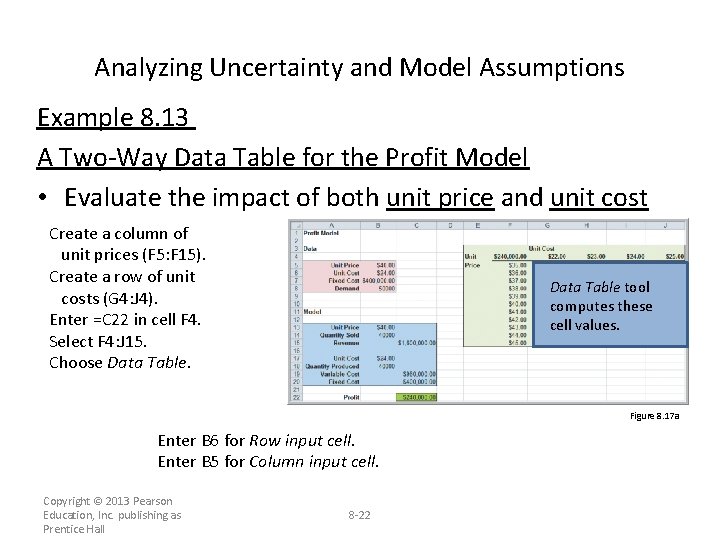
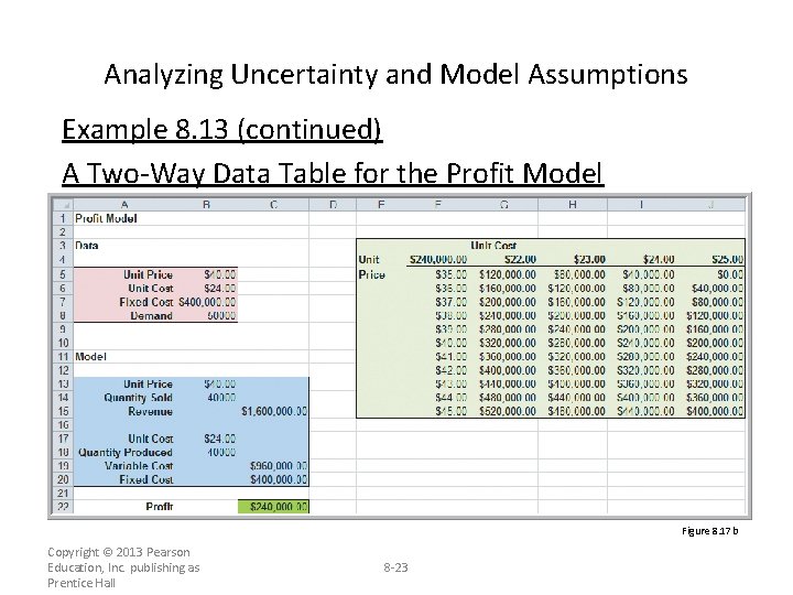
Analyzing Uncertainty and Model Assumptions Example 8. 13 A Two-Way Data Table for the Profit Model • Evaluate the impact of both unit price and unit cost Create a column of unit prices (F 5: F 15). Create a row of unit costs (G 4: J 4). Enter =C 22 in cell F 4. Select F 4: J 15. Choose Data Table tool computes these cell values. Figure 8. 17 a Enter B 6 for Row input cell. Enter B 5 for Column input cell. Copyright © 2013 Pearson Education, Inc. publishing as Prentice Hall 8 -22

Analyzing Uncertainty and Model Assumptions Example 8. 13 (continued) A Two-Way Data Table for the Profit Model Figure 8. 17 b Copyright © 2013 Pearson Education, Inc. publishing as Prentice Hall 8 -23

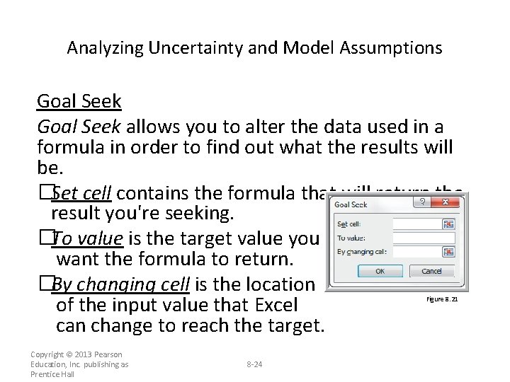
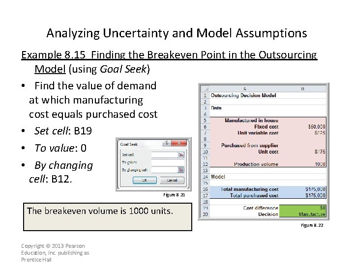
Analyzing Uncertainty and Model Assumptions Goal Seek allows you to alter the data used in a formula in order to find out what the results will be. �Set cell contains the formula that will return the result you're seeking. �To value is the target value you want the formula to return. �By changing cell is the location of the input value that Excel can change to reach the target. Figure 8. 21 Copyright © 2013 Pearson Education, Inc. publishing as Prentice Hall 8 -24

Analyzing Uncertainty and Model Assumptions Example 8. 15 Finding the Breakeven Point in the Outsourcing Model (using Goal Seek) • Find the value of demand at which manufacturing cost equals purchased cost • Set cell: B 19 • To value: 0 • By changing cell: B 12. Figure 8. 21 The breakeven volume is 1000 units. Figure 8. 22 Copyright © 2013 Pearson Education, Inc. publishing as Prentice Hall