Predictive Methods and Development of Statistical Models Part

Predictive Methods and Development of Statistical Models– Part II Fall 2019

Crash-Frequency Models Count Data Models Lord, D. , and F. Mannering (2010) The Statistical Analysis of Crash-Frequency Data: A Review and Assessment of Methodological Alternatives. Transportation Research - Part A, Vol. 44, No. 5, pp. 291 -305. Mannering, F. , Bhat, C. R. , 2014. Analytic methods in accident research: methodological frontier and future directions. Analytic Methods in Accident Research 1, 1 -22.

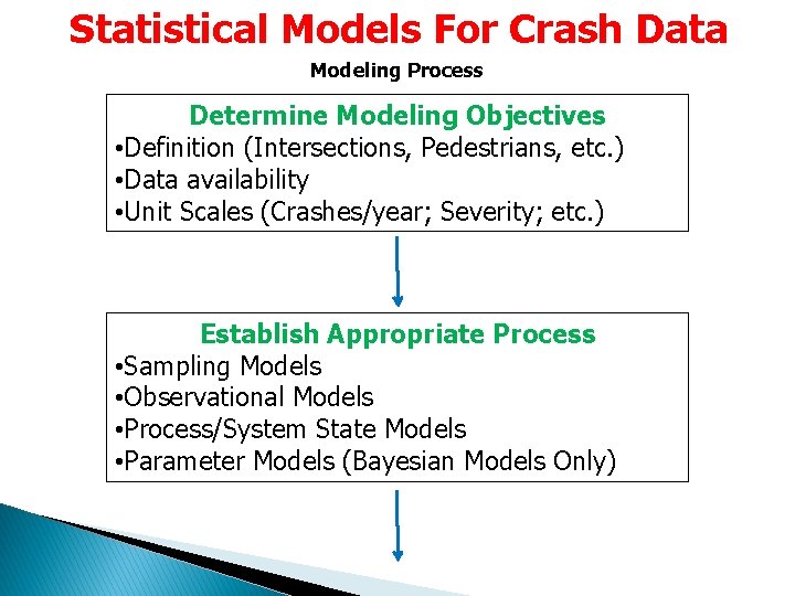
Statistical Models For Crash Data Modeling Process Determine Modeling Objectives • Definition (Intersections, Pedestrians, etc. ) • Data availability • Unit Scales (Crashes/year; Severity; etc. ) Establish Appropriate Process • Sampling Models • Observational Models • Process/System State Models • Parameter Models (Bayesian Models Only)

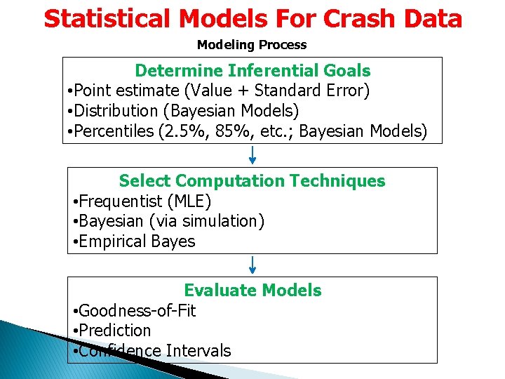
Statistical Models For Crash Data Modeling Process Determine Inferential Goals • Point estimate (Value + Standard Error) • Distribution (Bayesian Models) • Percentiles (2. 5%, 85%, etc. ; Bayesian Models) Select Computation Techniques • Frequentist (MLE) • Bayesian (via simulation) • Empirical Bayes Evaluate Models • Goodness-of-Fit • Prediction • Confidence Intervals

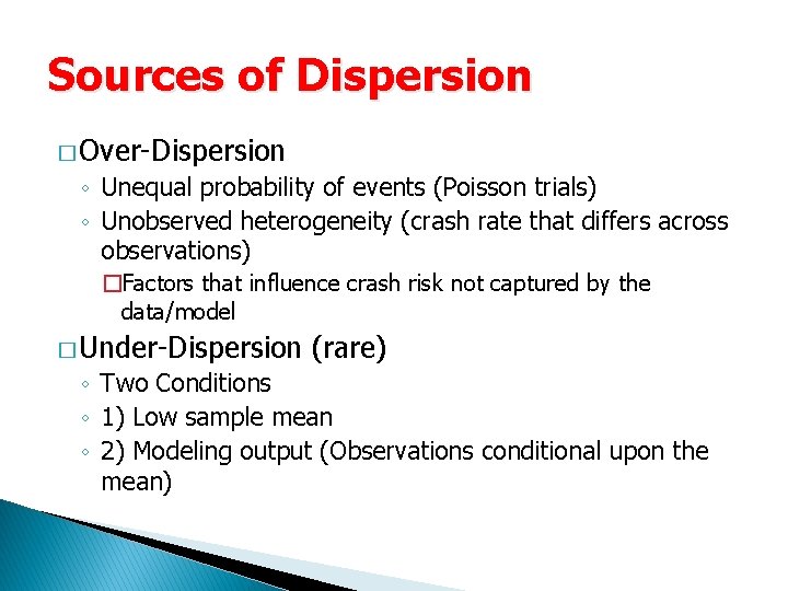
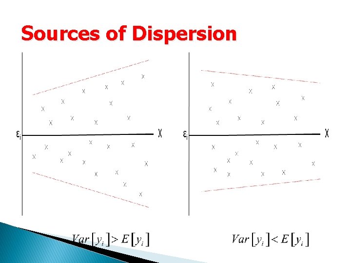
Sources of Dispersion � Over-Dispersion ◦ Unequal probability of events (Poisson trials) ◦ Unobserved heterogeneity (crash rate that differs across observations) �Factors that influence crash risk not captured by the data/model � Under-Dispersion (rare) ◦ Two Conditions ◦ 1) Low sample mean ◦ 2) Modeling output (Observations conditional upon the mean)

Sources of Dispersion

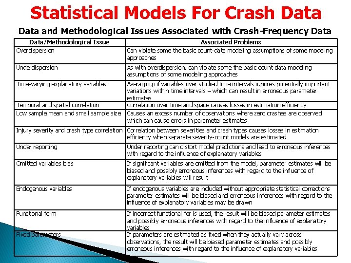
Statistical Models For Crash Data and Methodological Issues Associated with Crash-Frequency Data/Methodological Issue Overdispersion Associated Problems Can violate some the basic count-data modeling assumptions of some modeling approaches Underdispersion As with overdispersion, can violate some the basic count-data modeling assumptions of some modeling approaches Time-varying explanatory variables Averaging of variables over studied time intervals ignores potentially important variations within time intervals – which can result in erroneous parameter estimates Correlation over time and space causes losses in estimation efficiency Causes an excess number of observations where zero crashes are observed which can cause errors in parameter estimates Temporal and spatial correlation Low sample mean and small sample size Injury severity and crash type correlation Correlation between severities and crash types causes losses in estimation efficiency when separate severity-count models are estimated Under reporting can distort model predictions and lead to erroneous inferences with regard to the influence of explanatory variables Omitted variables bias If significant variables are omitted from the model, parameter estimates will be biased and possibly erroneous inferences with regard to the influence of explanatory variables will result Endogenous variables If endogenous variables are included without appropriate statistical corrections parameter estimates will be biased and erroneous inferences with regard to the influence of explanatory variables may be drawn Functional form If incorrect functional for is used, the result will be biased parameter estimates and possibly erroneous inferences with regard to the influence of explanatory variables If parameters are estimated as fixed when they actually vary across observations, the result will be biased parameter estimates and possibly erroneous inferences with regard to the influence of explanatory variables Fixed parameters

Basic Nomenclature is the response variable for observation i. is a p x 1 vector of estimable parameters. is a vector of explanatory variables. is the number of parameters in the model. is a random error term of the model.

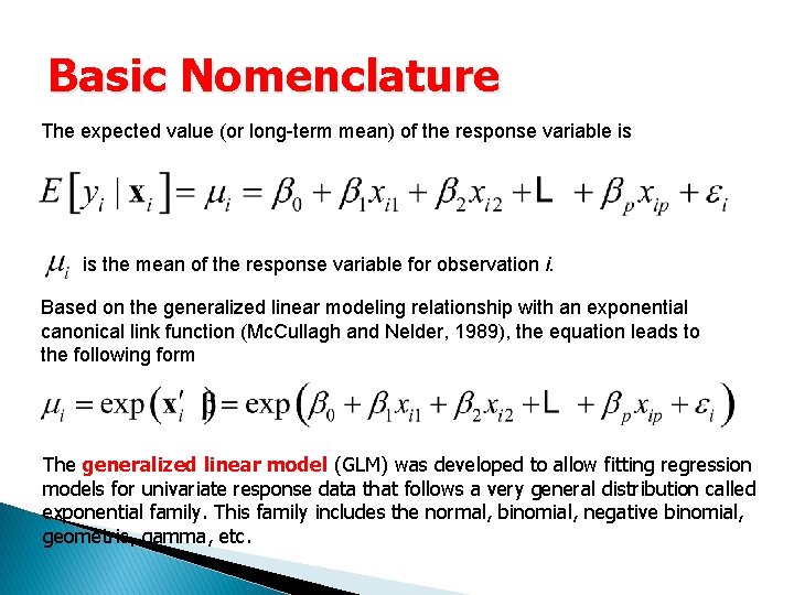
Basic Nomenclature The expected value (or long-term mean) of the response variable is is the mean of the response variable for observation i. Based on the generalized linear modeling relationship with an exponential canonical link function (Mc. Cullagh and Nelder, 1989), the equation leads to the following form The generalized linear model (GLM) was developed to allow fitting regression models for univariate response data that follows a very general distribution called exponential family. This family includes the normal, binomial, negative binomial, geometric, gamma, etc.

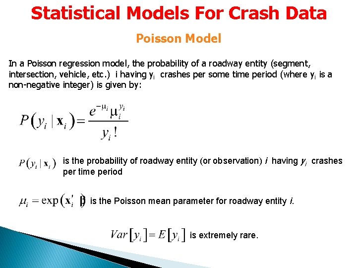
Statistical Models For Crash Data Poisson Model In a Poisson regression model, the probability of a roadway entity (segment, intersection, vehicle, etc. ) i having yi crashes per some time period (where yi is a non-negative integer) is given by: is the probability of roadway entity (or observation) i having yi crashes per time period is the Poisson mean parameter for roadway entity i. is extremely rare.

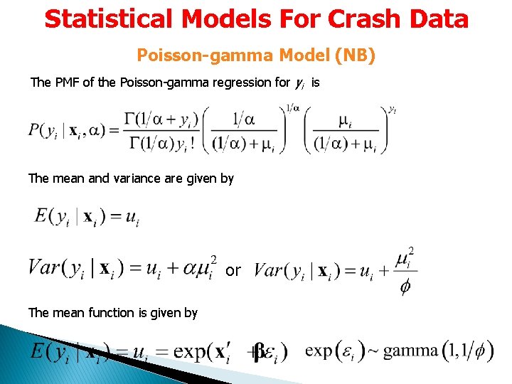
Statistical Models For Crash Data Poisson-gamma Model (NB) The PMF of the Poisson-gamma regression for yi is The mean and variance are given by or The mean function is given by

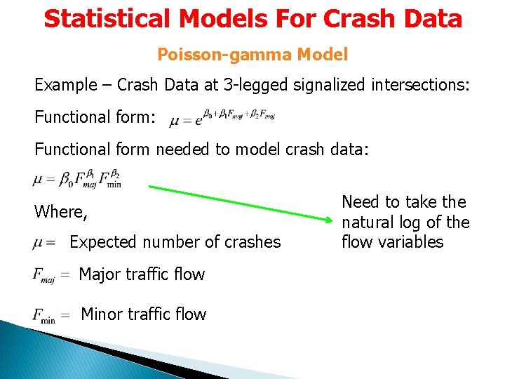
Statistical Models For Crash Data Poisson-gamma Model Example – Crash Data at 3 -legged signalized intersections: Functional form needed to model crash data: Where, Expected number of crashes Major traffic flow Minor traffic flow Need to take the natural log of the flow variables

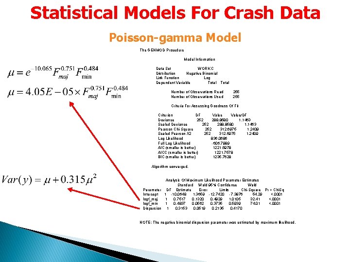
Statistical Models For Crash Data Poisson-gamma Model The GENMOD Procedure Model Information Data Set WORK. C Distribution Negative Binomial Link Function Log Dependent Variable Total Number of Observations Read 255 Number of Observations Used 255 Criteria For Assessing Goodness Of Fit Criterion DF Value/DF Deviance 252 288. 8580 1. 1463 Scaled Deviance 252 288. 8580 1. 1463 Pearson Chi-Square 252 312. 6975 1. 2409 Scaled Pearson X 2 252 312. 6975 1. 2409 Log Likelihood 836. 0686 Full Log Likelihood -606. 7989 AIC (smaller is better) 1221. 5978 AICC (smaller is better) 1221. 7578 BIC (smaller is better) 1235. 7628 Algorithm converged. Analysis Of Maximum Likelihood Parameter Estimates Standard Wald 95% Confidence Wald Parameter DF Estimate Error Limits Chi-Square Pr > Chi. Sq Intercept 1 -10. 0648 1. 3659 -12. 7420 -7. 3876 54. 29 <. 0001 logf_maj 1 0. 7517 0. 1320 0. 4929 1. 0105 32. 41 <. 0001 logf_min 1 0. 4837 0. 0562 0. 3735 0. 5939 74. 01 <. 0001 Dispersion 1 0. 3153 0. 0519 0. 2135 0. 4170 NOTE: The negative binomial dispersion parameter was estimated by maximum likelihood.

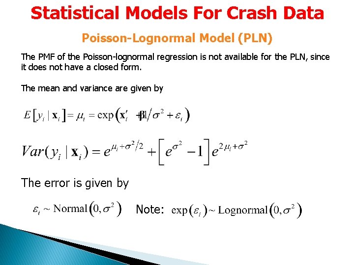
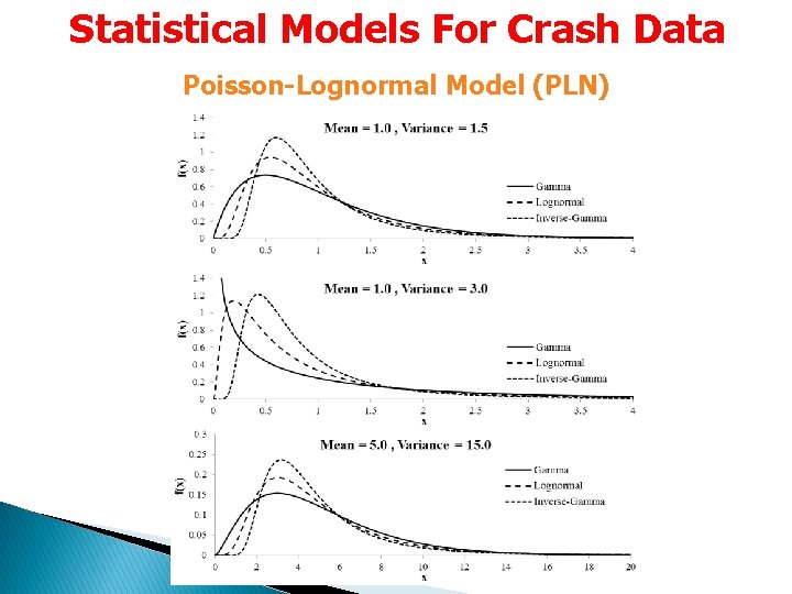
Statistical Models For Crash Data Poisson-Lognormal Model (PLN) The PMF of the Poisson-lognormal regression is not available for the PLN, since it does not have a closed form. The mean and variance are given by The error is given by Note:

Statistical Models For Crash Data Poisson-Lognormal Model (PLN)

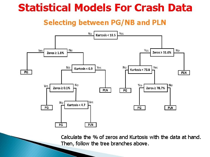
Statistical Models For Crash Data Selecting between PG/NB and PLN Calculate the % of zeros and Kurtosis with the data at hand. Then, follow the tree branches above.

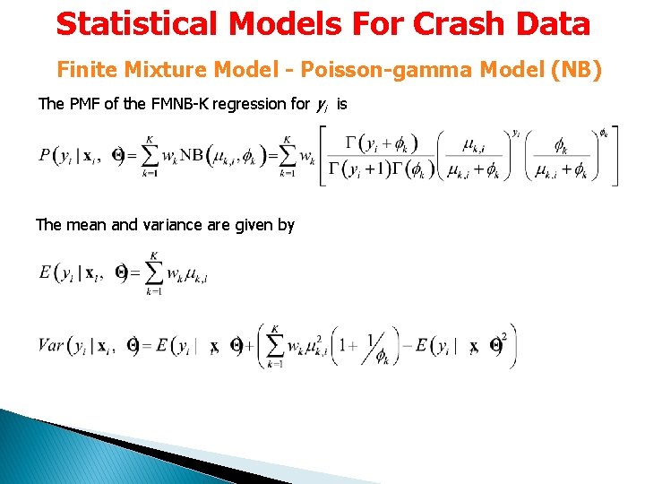
Statistical Models For Crash Data Finite Mixture Model - Poisson-gamma Model (NB) The PMF of the FMNB-K regression for yi is The mean and variance are given by

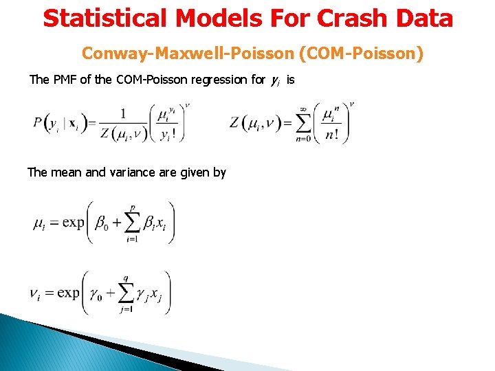
Statistical Models For Crash Data Conway-Maxwell-Poisson (COM-Poisson) The PMF of the COM-Poisson regression for yi is The mean and variance are given by

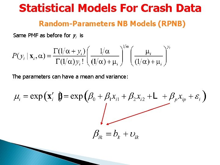
Statistical Models For Crash Data Random-Parameters NB Models (RPNB) Same PMF as before for yi is The parameters can have a mean and variance:

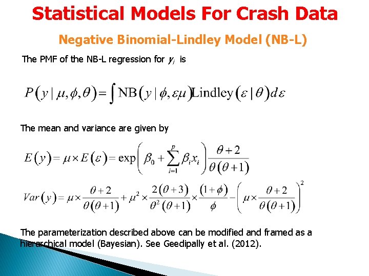
Statistical Models For Crash Data Negative Binomial-Lindley Model (NB-L) The PMF of the NB-L regression for yi is The mean and variance are given by The parameterization described above can be modified and framed as a hierarchical model (Bayesian). See Geedipally et al. (2012).

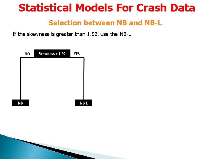
Statistical Models For Crash Data Selection between NB and NB-L If the skewness is greater than 1. 92, use the NB-L:

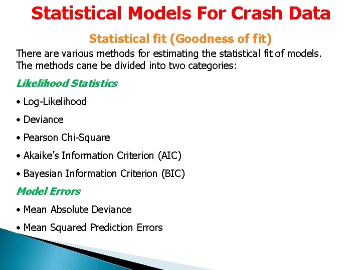
Statistical Models For Crash Data Statistical fit (Goodness of fit) There are various methods for estimating the statistical fit of models. The methods cane be divided into two categories: Likelihood Statistics • Log-Likelihood • Deviance • Pearson Chi-Square • Akaike’s Information Criterion (AIC) • Bayesian Information Criterion (BIC) Model Errors • Mean Absolute Deviance • Mean Squared Prediction Errors

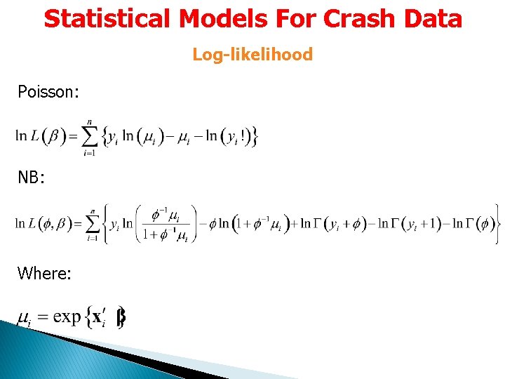
Statistical Models For Crash Data Log-likelihood Poisson: NB: Where:

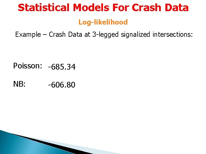
Statistical Models For Crash Data Log-likelihood Example – Crash Data at 3 -legged signalized intersections: Poisson: -685. 34 NB: -606. 80

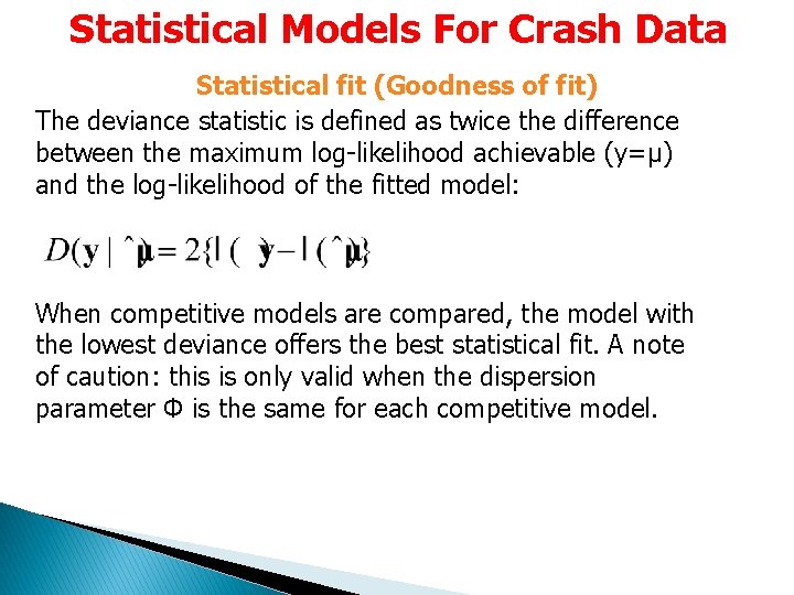
Statistical Models For Crash Data Statistical fit (Goodness of fit) The deviance statistic is defined as twice the difference between the maximum log-likelihood achievable (y=μ) and the log-likelihood of the fitted model: When competitive models are compared, the model with the lowest deviance offers the best statistical fit. A note of caution: this is only valid when the dispersion parameter Φ is the same for each competitive model.

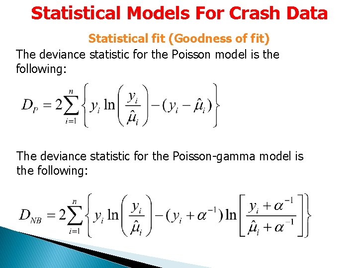
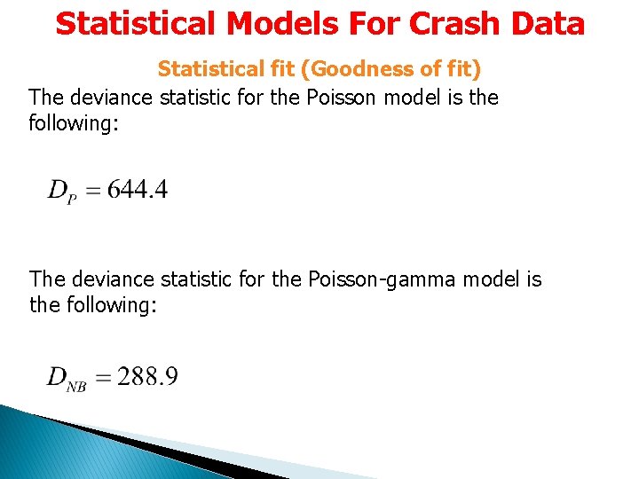
Statistical Models For Crash Data Statistical fit (Goodness of fit) The deviance statistic for the Poisson model is the following: The deviance statistic for the Poisson-gamma model is the following:

Statistical Models For Crash Data Statistical fit (Goodness of fit) The deviance statistic for the Poisson model is the following: The deviance statistic for the Poisson-gamma model is the following:

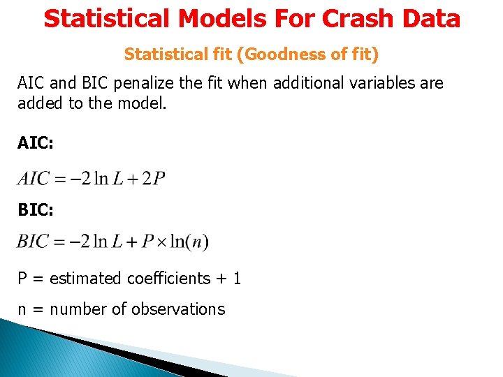
Statistical Models For Crash Data Statistical fit (Goodness of fit) AIC and BIC penalize the fit when additional variables are added to the model. AIC: BIC: P = estimated coefficients + 1 n = number of observations

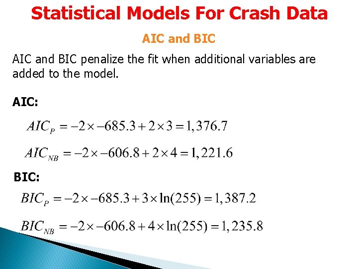
Statistical Models For Crash Data AIC and BIC penalize the fit when additional variables are added to the model. AIC: BIC:

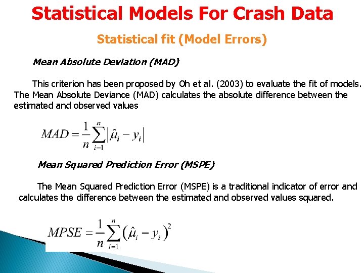
Statistical Models For Crash Data Statistical fit (Model Errors) Mean Absolute Deviation (MAD) This criterion has been proposed by Oh et al. (2003) to evaluate the fit of models. The Mean Absolute Deviance (MAD) calculates the absolute difference between the estimated and observed values Mean Squared Prediction Error (MSPE) The Mean Squared Prediction Error (MSPE) is a traditional indicator of error and calculates the difference between the estimated and observed values squared.

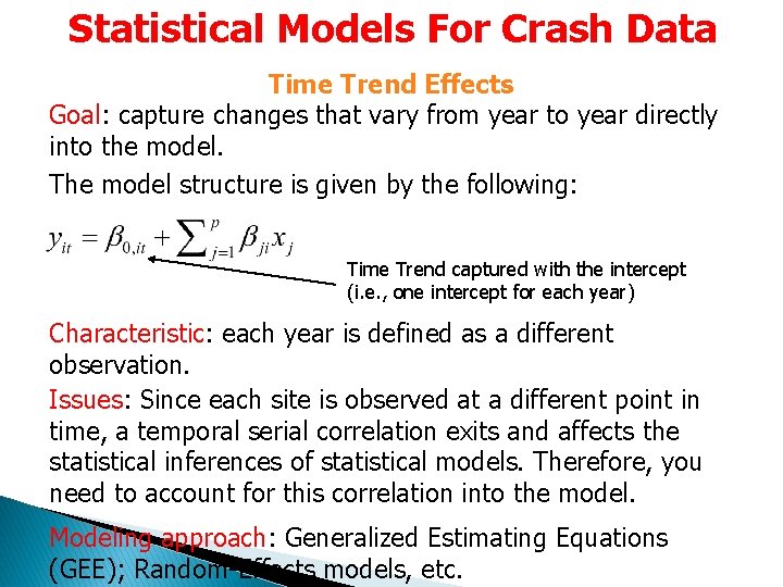
Statistical Models For Crash Data Time Trend Effects Goal: capture changes that vary from year to year directly into the model. The model structure is given by the following: Time Trend captured with the intercept (i. e. , one intercept for each year) Characteristic: each year is defined as a different observation. Issues: Since each site is observed at a different point in time, a temporal serial correlation exits and affects the statistical inferences of statistical models. Therefore, you need to account for this correlation into the model. Modeling approach: Generalized Estimating Equations (GEE); Random-Effects models, etc.

Bayes Methods � The Bayes method approaches the analysis of data differently than the classical method (frequentist) � Subjective judgment more easily incorporated with the observed data and models � Treat unknown coefficients of regression models as random variables � Data analysis less limited by the number of observations (can be supplemented with subjective judgment) � Computationally intensive (no longer an issue)

Bayes Methods � The Bayes method makes inferences from data using probability models for quantities that are observed and for quantities one is interested to learn about � Bayesian data analysis can be divided into three steps: ◦ Setting up a full probability model: provide a joint probability distribution for all observable and unobservable quantities ◦ Conditioning on observed data: calculating and interpreting the appropriate posterior distribution (conditional probability distribution) ◦ Evaluating the fit of the model and implication of the posterior distribution � Emphasis placed on interval estimation (confidence interval) rather than hypothesis testing

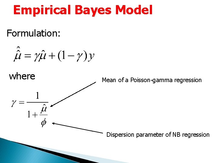
Empirical Bayes Model � For the EB method, a different weight is assigned to the prior distribution and standard estimate respectively � In safety analyses, the weights are estimated with the assumption that the mean () for each site follows a Gamma distribution � The EB estimates has been found to outperform other estimates, such as the MLE � The EB framework is presented on next overhead

Empirical Bayes Model Formulation: where Mean of a Poisson-gamma regression Dispersion parameter of NB regression

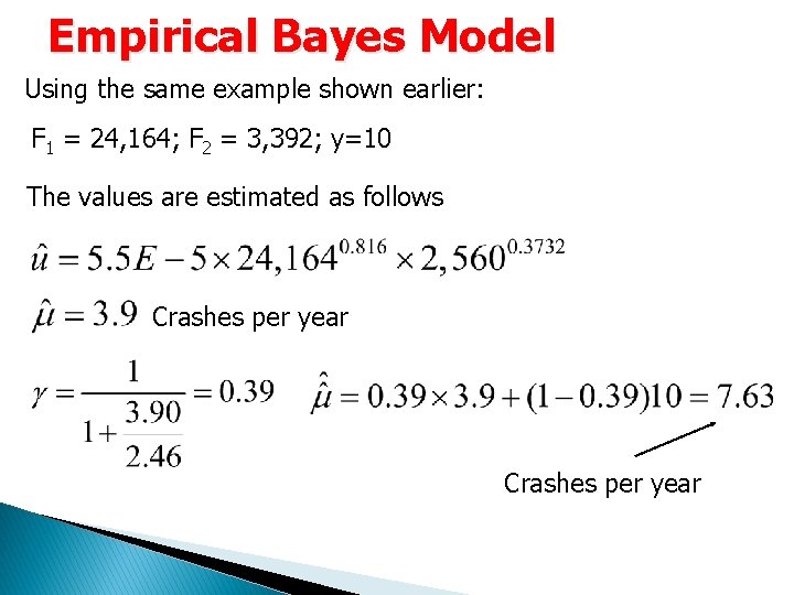
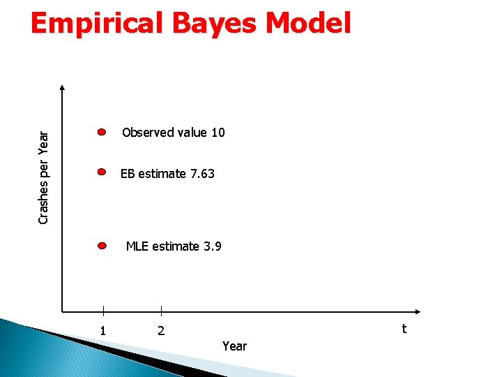
Empirical Bayes Model Using the same example shown earlier: F 1 = 24, 164; F 2 = 3, 392; y=10 The values are estimated as follows Crashes per year

Empirical Bayes Model Crashes per Year Observed value 10 EB estimate 7. 63 MLE estimate 3. 9 1 t 2 Year

Crash-Severity Models (Discrete Choice Models) Savolainen, P. T. , F. L. Mannering, D. Lord, and M. A. Quddus (2011) The Statistical Analysis of Highway Crash-Injury Severities: A Review and Assessment of Methodological Alternatives. Accident Analysis & Prevention, Vol. 43, No. 5, pp. 1666 -1676. Ivan, J. N. , and K. C. Konduri (2018) Crash Severity Methods. Chapter 15 in Safe Mobility: Challenges, Methodology and Solutions. Emerald Publishing Limited,

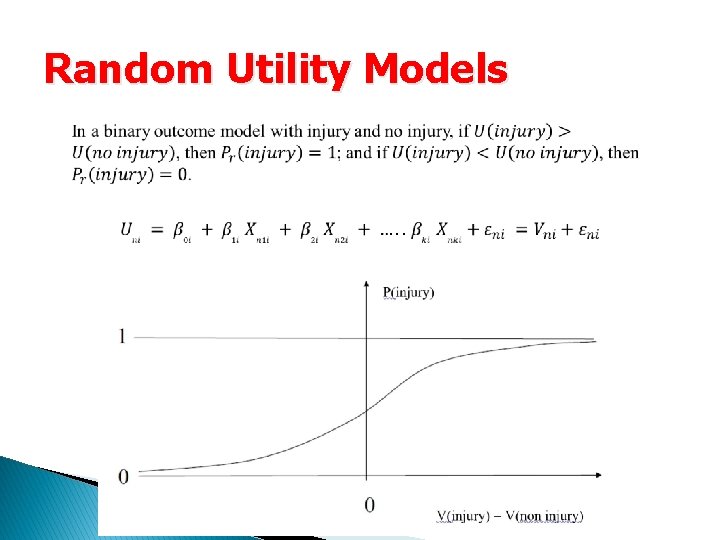
Random Utility Models

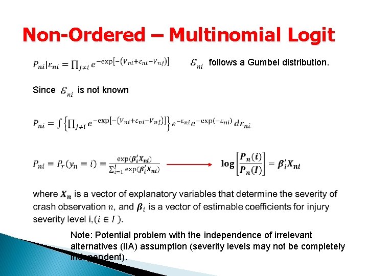
Non-Ordered – Multinomial Logit follows a Gumbel distribution. Since is not known Note: Potential problem with the independence of irrelevant alternatives (IIA) assumption (severity levels may not be completely independent).

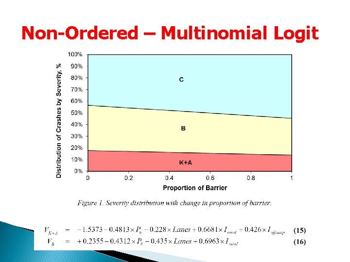
Non-Ordered – Multinomial Logit

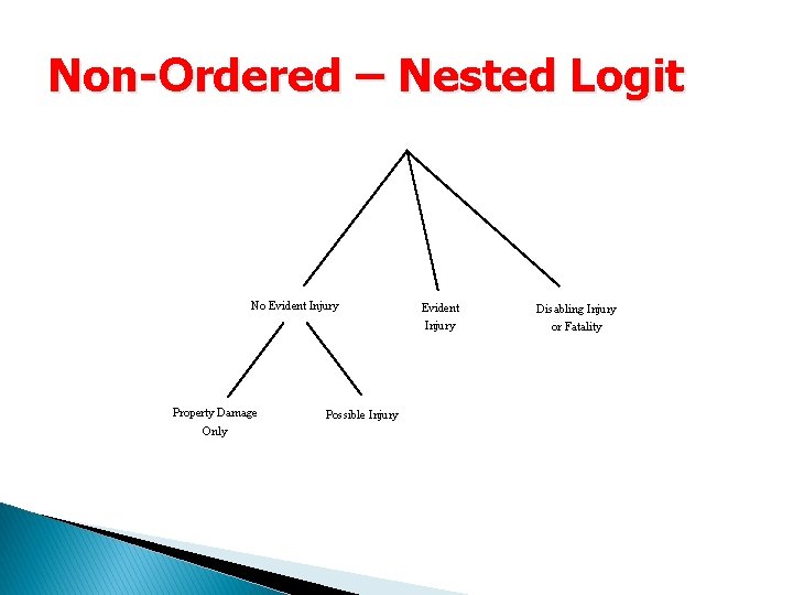
Non-Ordered – Nested Logit No Evident Injury Property Damage Only Possible Injury Evident Injury Disabling Injury or Fatality

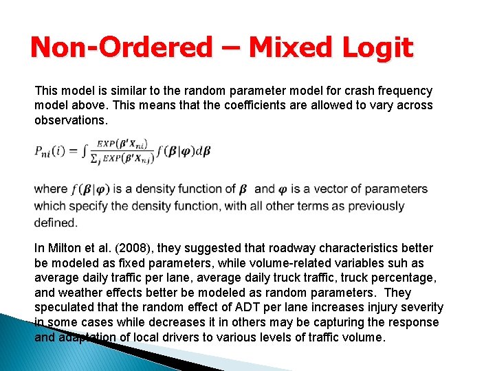
Non-Ordered – Mixed Logit This model is similar to the random parameter model for crash frequency model above. This means that the coefficients are allowed to vary across observations. In Milton et al. (2008), they suggested that roadway characteristics better be modeled as fixed parameters, while volume-related variables suh as average daily traffic per lane, average daily truck traffic, truck percentage, and weather effects better be modeled as random parameters. They speculated that the random effect of ADT per lane increases injury severity in some cases while decreases it in others may be capturing the response and adaptation of local drivers to various levels of traffic volume.

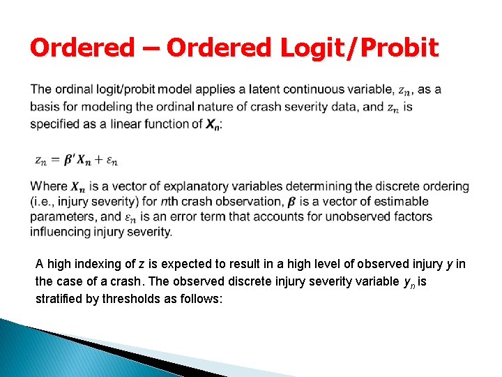
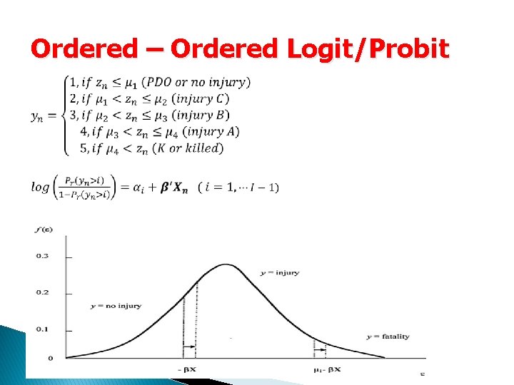
Ordered – Ordered Logit/Probit A high indexing of z is expected to result in a high level of observed injury y in the case of a crash. The observed discrete injury severity variable yn is stratified by thresholds as follows:

Ordered – Ordered Logit/Probit

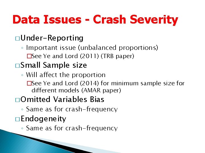
Data Issues - Crash Severity � Under-Reporting ◦ Important issue (unbalanced proportions) �See Ye and Lord (2011) (TRB paper) � Small Sample size ◦ Will affect the proportion �See Ye and Lord (2014) for minimum sample size for different models (AMAR paper) � Omitted Variables Bias ◦ Same as for crash-frequency � Endogeneity ◦ Same as for crash-frequency