Predictive Analytics for Data Mining Regression Classification Weifeng

Predictive Analytics for Data Mining: Regression & Classification Weifeng Li, Sagar Samtani, and Hsinchun Chen Spring 2020 Acknowledgements: Cynthia Rudin, Hastie & Tibshirani Michael Crawford – San Jose State University Pier Luca Lanzi – Politecnico di Milano John Whitehead, East Carolina University 1

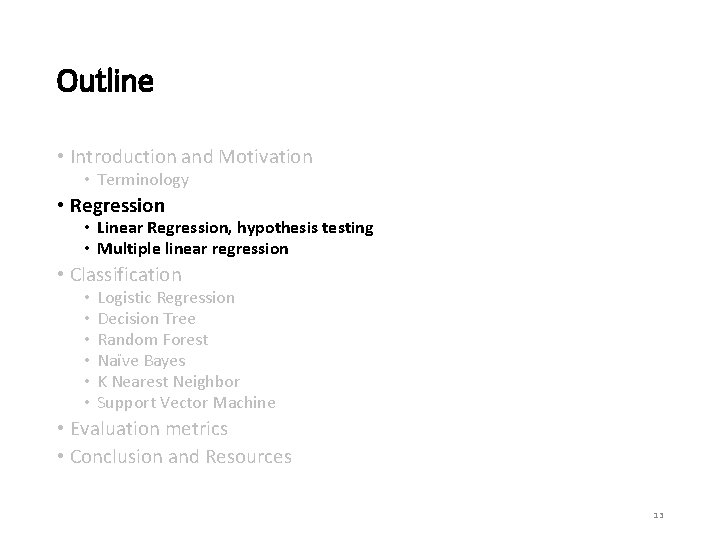
Outline • Introduction and Motivation • Terminology • Top DM methods and tools • Regression • Linear Regression, hypothesis testing • Multiple linear regression • Classification • • • Logistic Regression Decision Tree Random Forest Naïve Bayes K Nearest Neighbor Support Vector Machine • Evaluation metrics • Conclusion and Resources 2

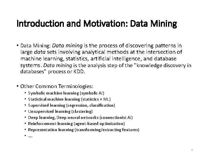
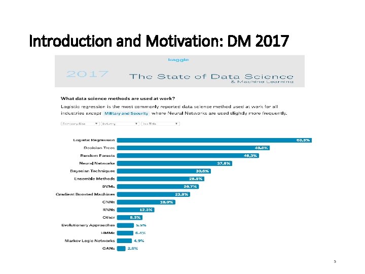
Introduction and Motivation: Data Mining • Data Mining: Data mining is the process of discovering patterns in large data sets involving analytical methods at the intersection of machine learning, statistics, artificial intelligence, and database systems. Data mining is the analysis step of the "knowledge discovery in databases" process or KDD. • Other Common Terminologies: • • Symbolic machine learning (symbolic AI) Statistical machine learning (statistics + ML) Supervised learning (regression, classification) Unsupervised learning (clustering) Deep learning, Deep neural networks (connectionist AI) Reinforcement learning (agent-based optimization) Representation learning (transforming/extracting features) …. 3

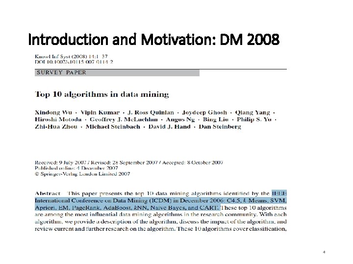
Introduction and Motivation: DM 2008 4

Introduction and Motivation: DM 2017 5

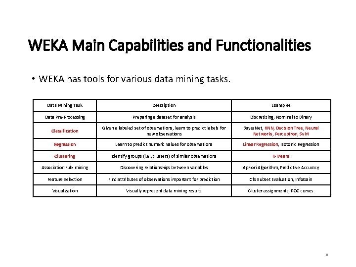
WEKA Main Capabilities and Functionalities • WEKA has tools for various data mining tasks. Data Mining Task Description Examples Data Pre-Processing Preparing a dataset for analysis Discretizing, Nominal to Binary Classification Given a labeled set of observations, learn to predict labels for new observations Bayes. Net, KNN, Decision Tree, Neural Networks, Perceptron, SVM Regression Learn to predict numeric values for observations Linear Regression, Isotonic Regression Clustering Identify groups (i. e. , clusters) of similar observations K-Means Association rule mining Discovering relationships between variables Apriori Algorithm, Predictive Accuracy Feature Selection Find attributes of observations important for prediction Cfs Subset Evaluation, Info. Gain Visualization Visually represent data mining results Cluster assignments, ROC curves 6

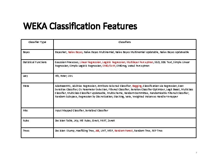
WEKA Classification Features Classifier Type Classifiers Bayes. Net, Naïve Bayes Multinomial, Naïve Bayes Multinomial Updatable, Naïve Bayes Updateable Statistical Functions Gaussian Processes, Linear Regression, Logistic Regression, Multilayer Perceptron, SGD, SDG Text, Simple Linear Regression, Simple Logistic Regression, SMO/SVM, SMOreg, Voted Perceptron Lazy IBk, Kstar, LWL Meta Ada. Boost. M 1, Additive Regression, Attribute Selected Classifier, Bagging, Classification via Regression, Cost Sensitive Classifier, CV Parameter Selection, Filtered Classifier, Iterative Classifier Optimizer, Logit Boost, Multiclass Classifier Updateable, Multischeme, Random Committee, Randomizable Filtered Classifier, Random Subspace, Regression by Discretization, Stacking, Vote, Weighted Instances Handler Wrapper Misc Input Mapped Classifier, Serialized Classifier Rules Decision Table, Jrip, M 5 Rules, One. R, PART, Zero. R Trees Decision Stump, Hoeffding Tree, J 48, LMT, M 5 P, Random Forest, Random Tree, REP Tree 7

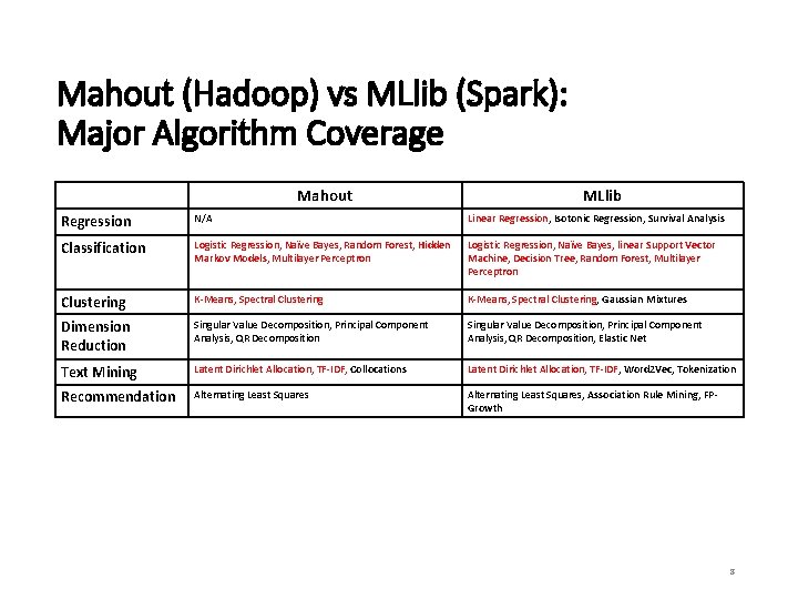
Mahout (Hadoop) vs MLlib (Spark): Major Algorithm Coverage Mahout MLlib Regression N/A Linear Regression, Isotonic Regression, Survival Analysis Classification Logistic Regression, Naïve Bayes, Random Forest, Hidden Markov Models, Multilayer Perceptron Logistic Regression, Naïve Bayes, linear Support Vector Machine, Decision Tree, Random Forest, Multilayer Perceptron Clustering K-Means, Spectral Clustering, Gaussian Mixtures Dimension Reduction Singular Value Decomposition, Principal Component Analysis, QR Decomposition, Elastic Net Text Mining Latent Dirichlet Allocation, TF-IDF, Collocations Latent Dirichlet Allocation, TF-IDF, Word 2 Vec, Tokenization Recommendation Alternating Least Squares, Association Rule Mining, FPGrowth 8

Introduction and Motivation: Predictive Analytics • In recent years, there has been a growing emphasis for researchers and practitioners alike to be able to “predict” the future based on past data. • These slides present two standard “predictive analytics” approaches: • Regression – given a set of attributes, predict the value for a record • Classification – given a set of attributes, predict the label (i. e. , class) for the record 9

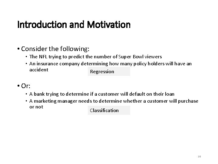
Introduction and Motivation • Consider the following: • The NFL trying to predict the number of Super Bowl viewers • An insurance company determining how many policy holders will have an accident Regression • Or: • A bank trying to determine if a customer will default on their loan • A marketing manager needs to determine whether a customer will purchase or not Classification 10

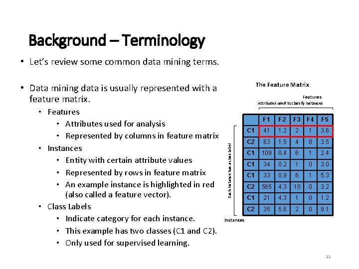
Background – Terminology • Let’s review some common data mining terms. The Feature Matrix • Data mining data is usually represented with a feature matrix. Each instance has a class label • Features • Attributes used for analysis • Represented by columns in feature matrix • Instances • Entity with certain attribute values • Represented by rows in feature matrix • An example instance is highlighted in red (also called a feature vector). • Class Labels • Indicategory for each instance. • This example has two classes (C 1 and C 2). • Only used for supervised learning. Features Attributes used to classify instances F 1 F 2 F 3 F 4 F 5 C 1 41 1. 2 2 1 3. 6 C 2 63 1. 5 4 0 3. 5 C 1 109 0. 4 6 1 2. 4 C 1 34 0. 2 1 0 3. 0 C 1 33 0. 9 6 1 5. 3 C 2 565 4. 3 10 0 3. 2 C 1 21 4. 3 1 0 1. 2 C 2 35 5. 6 2 0 9. 1 Instances 11

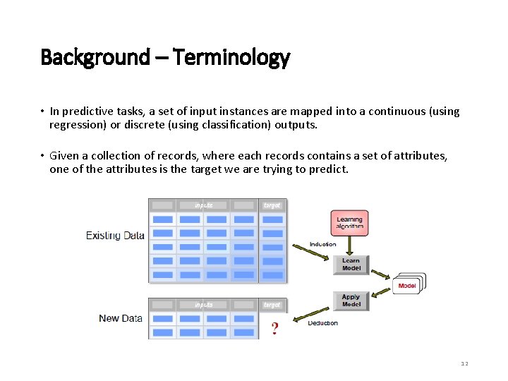
Background – Terminology • In predictive tasks, a set of input instances are mapped into a continuous (using regression) or discrete (using classification) outputs. • Given a collection of records, where each records contains a set of attributes, one of the attributes is the target we are trying to predict. 12

Outline • Introduction and Motivation • Terminology • Regression • Linear Regression, hypothesis testing • Multiple linear regression • Classification • • • Logistic Regression Decision Tree Random Forest Naïve Bayes K Nearest Neighbor Support Vector Machine • Evaluation metrics • Conclusion and Resources 13

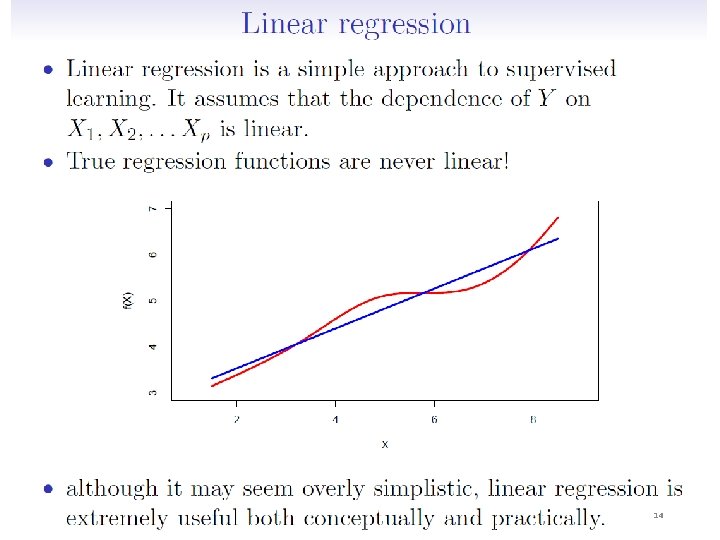
14

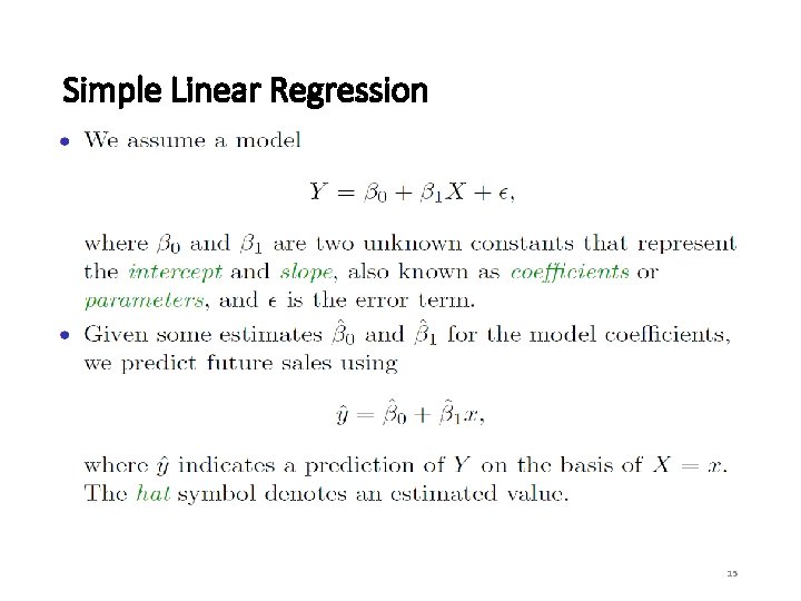
Simple Linear Regression 15

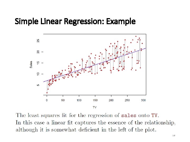
Simple Linear Regression: Example 16

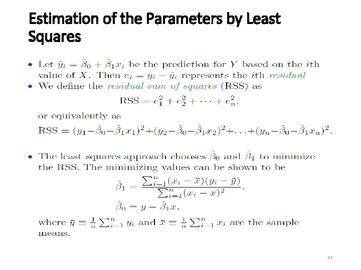
Estimation of the Parameters by Least Squares 17

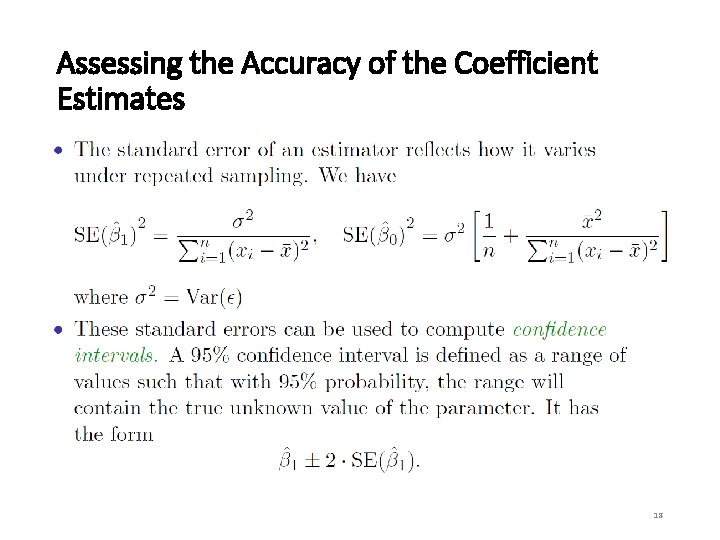
Assessing the Accuracy of the Coefficient Estimates 18

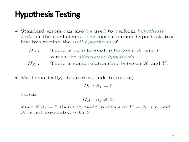
Hypothesis Testing 19

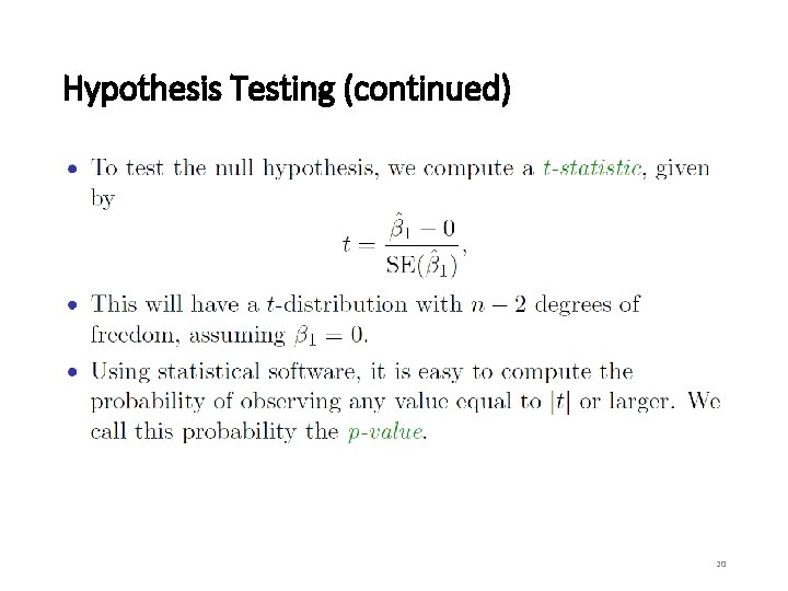
Hypothesis Testing (continued) 20

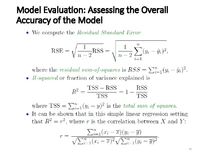
Model Evaluation: Assessing the Overall Accuracy of the Model 21

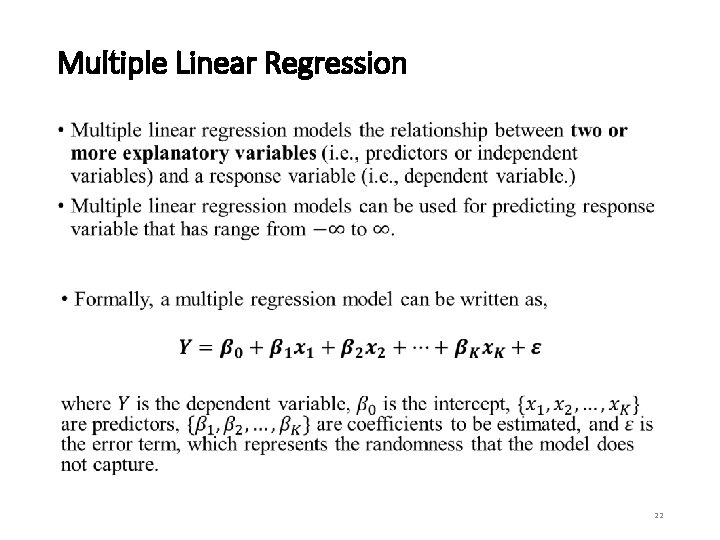
Multiple Linear Regression • 22

Outline • Introduction and Motivation • Terminology • Regression • Linear regression, hypothesis testing • Multiple linear regression • Classification • • • Logistic Regression Decision Tree Random Forest Naïve Bayes K Nearest Neighbor Support Vector Machine • Evaluation metrics • Conclusion and Resources 23

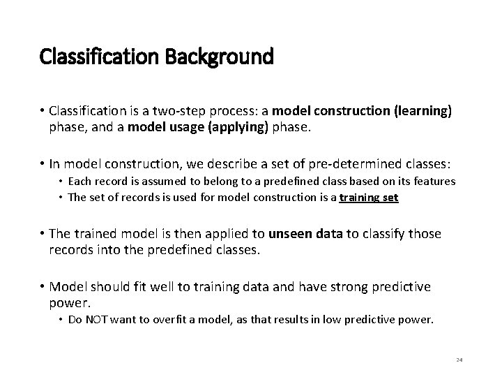
Classification Background • Classification is a two-step process: a model construction (learning) phase, and a model usage (applying) phase. • In model construction, we describe a set of pre-determined classes: • Each record is assumed to belong to a predefined class based on its features • The set of records is used for model construction is a training set • The trained model is then applied to unseen data to classify those records into the predefined classes. • Model should fit well to training data and have strong predictive power. • Do NOT want to overfit a model, as that results in low predictive power. 24

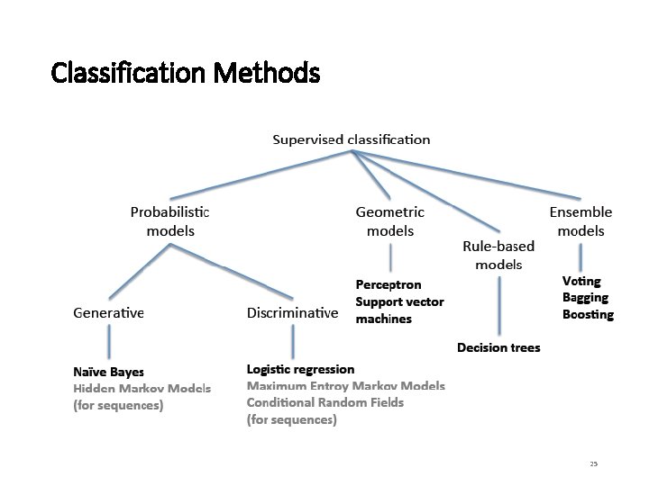
Classification Methods 25

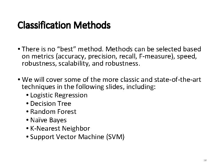
Classification Methods • There is no “best” method. Methods can be selected based on metrics (accuracy, precision, recall, F-measure), speed, robustness, scalability, and robustness. • We will cover some of the more classic and state-of-the-art techniques in the following slides, including: • Logistic Regression • Decision Tree • Random Forest • Naïve Bayes • K-Nearest Neighbor • Support Vector Machine (SVM) 26

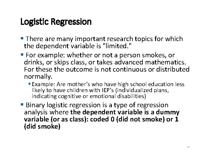
Logistic Regression § There are many important research topics for which the dependent variable is "limited. " § For example: whether or not a person smokes, or drinks, or skips class, or takes advanced mathematics. For these the outcome is not continuous or distributed normally. § Example: Are mother’s who have high school education less likely to have children with IEP’s (individualized plans, indicating cognitive or emotional disabilities) § Binary logistic regression is a type of regression analysis where the dependent variable is a dummy variable (or as class): coded 0 (did not smoke) or 1 (did smoke) 27

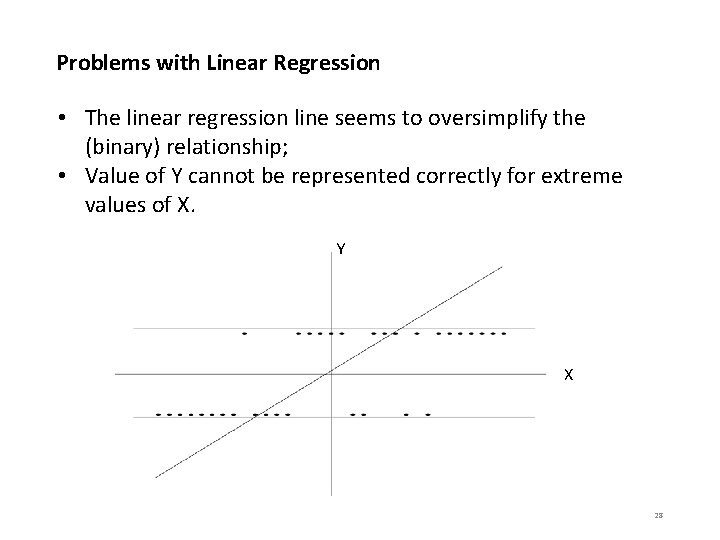
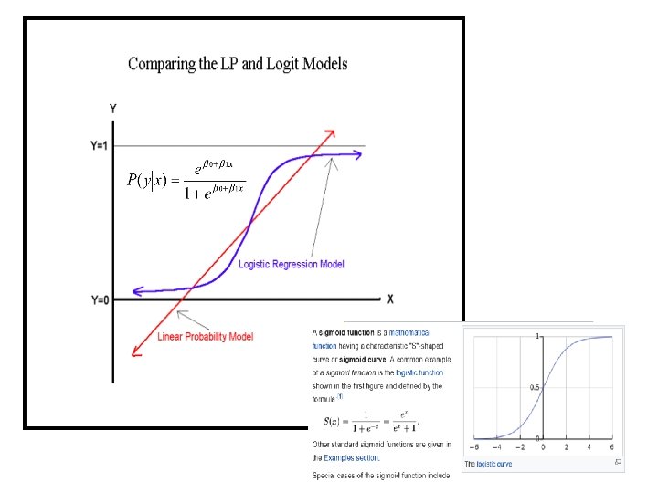
Problems with Linear Regression • The linear regression line seems to oversimplify the (binary) relationship; • Value of Y cannot be represented correctly for extreme values of X. Y X 28

29

The Logistic Regression Model The "logit" model solves these problems: ln[p/(1 -p)] = 0 + 1 X § p is the probability that the event Y occurs, p(Y=1) § [range=0 to 1] § p/(1 -p) is the "odds ratio" § [range=0 to ∞] § ln[p/(1 -p)]: log odds ratio, or "logit“ § [range=-∞ to +∞] 30

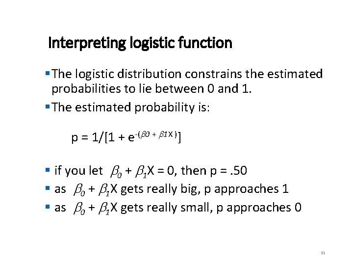
Interpreting logistic function §The logistic distribution constrains the estimated probabilities to lie between 0 and 1. §The estimated probability is: p = 1/[1 + e-( 0 + 1 X )] § if you let 0 + 1 X = 0, then p =. 50 § as 0 + 1 X gets really big, p approaches 1 § as 0 + 1 X gets really small, p approaches 0 31

Running Logistic Regression in SPSS ln[p/(1 -p)] = 0 + 1 X = -2. 424 -. 46 X 32

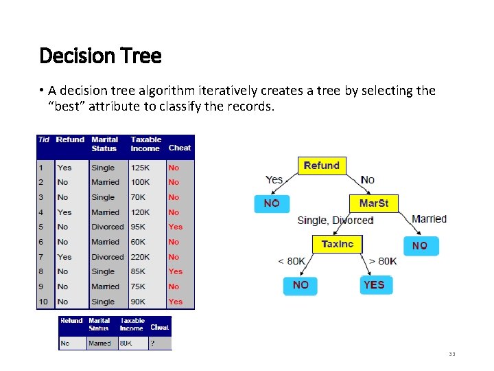
Decision Tree • A decision tree algorithm iteratively creates a tree by selecting the “best” attribute to classify the records. 33

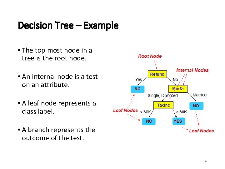
Decision Tree – Example • The top most node in a tree is the root node. • An internal node is a test on an attribute. • A leaf node represents a class label. • A branch represents the outcome of the test. 34

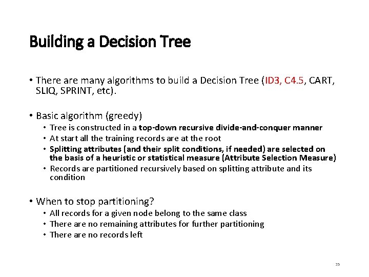
Building a Decision Tree • There are many algorithms to build a Decision Tree (ID 3, C 4. 5, CART, SLIQ, SPRINT, etc). • Basic algorithm (greedy) • Tree is constructed in a top-down recursive divide-and-conquer manner • At start all the training records are at the root • Splitting attributes (and their split conditions, if needed) are selected on the basis of a heuristic or statistical measure (Attribute Selection Measure) • Records are partitioned recursively based on splitting attribute and its condition • When to stop partitioning? • All records for a given node belong to the same class • There are no remaining attributes for further partitioning • There are no records left 35

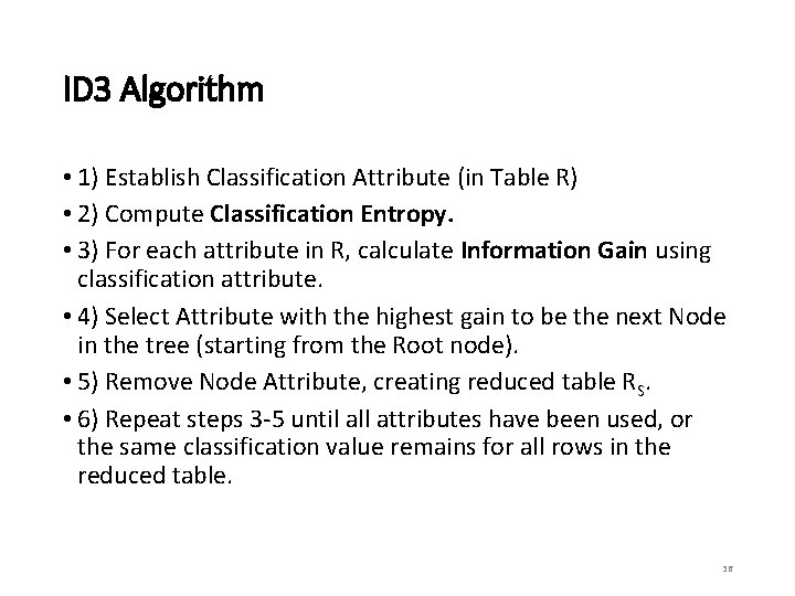
ID 3 Algorithm • 1) Establish Classification Attribute (in Table R) • 2) Compute Classification Entropy. • 3) For each attribute in R, calculate Information Gain using classification attribute. • 4) Select Attribute with the highest gain to be the next Node in the tree (starting from the Root node). • 5) Remove Node Attribute, creating reduced table RS. • 6) Repeat steps 3 -5 until all attributes have been used, or the same classification value remains for all rows in the reduced table. 36

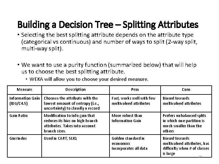
Building a Decision Tree – Splitting Attributes • Selecting the best splitting attribute depends on the attribute type (categorical vs continuous) and number of ways to split (2 -way split, multi-way split). • We want to use a purity function (summarized below) that will help us to choose the best splitting attribute. • WEKA will allow you to choose your desired measure. Measure Description Pros Cons Information Gain Chooses the attribute with the (ID 3/C 4. 5) lowest amount of entropy (i. e. , uncertainty) to classify a record Fast, works well with few multivalued attributes Biased towards multivalued attributes Gain Ratio Modification to Info gain that reduces its bias on high-branch attributes. Takes into account branch sizes. More robust than Information Gain Prefers unbalanced splits in which one partition is much smaller than the others Gini Index Used in CART, SLIQ Golden standard in economics Incorporates all data Biased towards multivalued attributes, has difficulty when # of classes is large 37

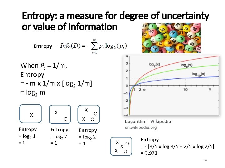
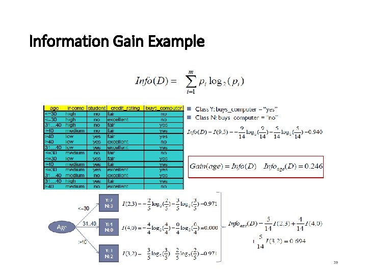
Entropy: a measure for degree of uncertainty or value of information Entropy = When Pi = 1/m, Entropy = - m x 1/m x [log 2 1/m] = log 2 m X Entropy = log 2 1 =0 X X O O X O Entropy = log 2 2 =1 X X O Entropy = - [3/5 x log 3/5 + 2/5 x log 2/5] = 0. 971 38

Information Gain Example 39

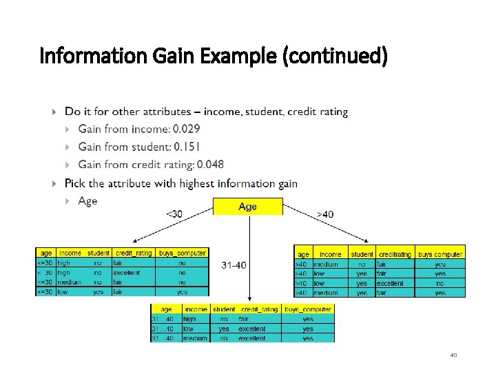
Information Gain Example (continued) 40

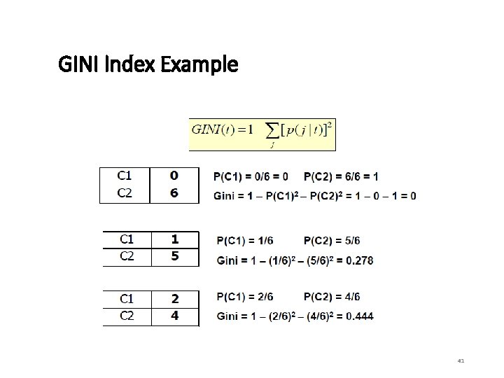
GINI Index Example 41

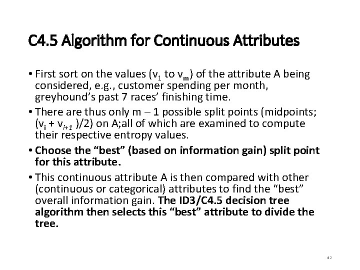
C 4. 5 Algorithm for Continuous Attributes • First sort on the values (v 1 to vm) of the attribute A being considered, e. g. , customer spending per month, greyhound’s past 7 races’ finishing time. • There are thus only m – 1 possible split points (midpoints; (vi + vi+1 )/2) on A; all of which are examined to compute their respective entropy values. • Choose the “best” (based on information gain) split point for this attribute. • This continuous attribute A is then compared with other (continuous or categorical) attributes to find the “best” overall information gain. The ID 3/C 4. 5 decision tree algorithm then selects this “best” attribute to divide the tree. 42

Building a Decision Tree - Pruning • A common issue with Decision Tree is overfitting. To address such an issue, we can apply pre and post-pruning rules. • WEKA will give you these options. • Pre-pruning – stop the algorithm before it becomes a full tree. Typical stopping conditions for a node include: • Stop if all records for a given node belong to the same class • Stop if there are no remaining attributes for further partitioning • Stop if there are no records left • Post-pruning – grow the tree to its entirety. • Trim the nodes of the tree in a bottom-up fashion • If error improves after trimming, replace sub-tree by a leaf node • Class label of leaf is determined from majority class of records in sub-tree 43

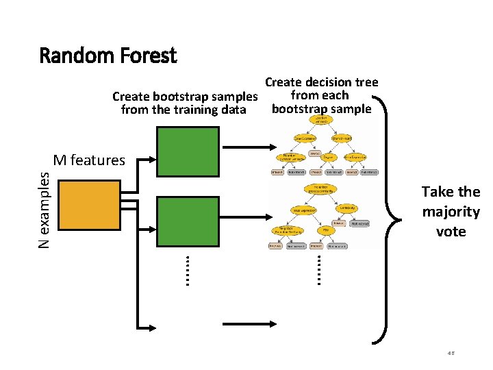
Random Forest – Bagging • Before Random Forest, we must first understand “bagging. ” • Bagging is the idea wherein a classifier is made up of many individual classifiers from the same family. • They are combined through majority rule (unweighted) • Each classifier is trained on a bootstrapped sample with replacement from the training data. • Each of classifiers in the bag is a “weak” classifier 44

Random Forest • Random Forest is based off of decision tree and bagging. • The weak classifier in Random Forest is a decision tree. • Each decision tree in the bag is using only a subset of features. • Only two hyper-parameters to tune: • How many trees to build • What percentage of features to use in each tree • Performs very well and can be implemented in WEKA! 45

Random Forest Create decision tree from each Create bootstrap samples bootstrap sample from the training data N examples M features . . . . … Take the majority vote 46

Naïve Bayes • Naïve Bayes is a probabilistic classifier applying Bayes’ theorem. • Assumes that the value of features are independent of other features and that features have equal importance. • Hence “Naive” • Scales and performs well in text categorization tasks. • E. g. , spam or legitimate email, sports or politics, etc. • Also has extensions such as Gaussian Naïve Bayes, Multinomial Naïve Bayes, and Bernoulli Naïve Bayes. • Naïve Bayes and Multinomial Naïve Bayes are part of WEKA 47

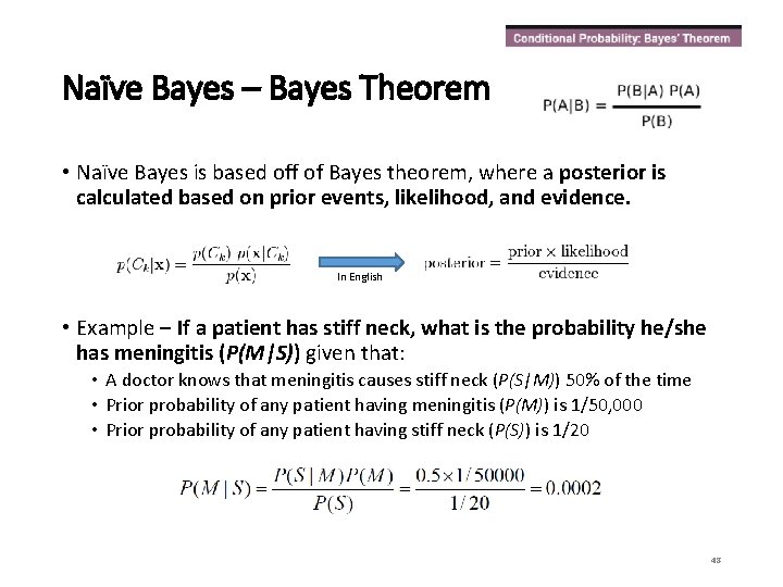
Naïve Bayes – Bayes Theorem • Naïve Bayes is based off of Bayes theorem, where a posterior is calculated based on prior events, likelihood, and evidence. In English • Example – If a patient has stiff neck, what is the probability he/she has meningitis (P(M|S)) given that: • A doctor knows that meningitis causes stiff neck (P(S|M)) 50% of the time • Prior probability of any patient having meningitis (P(M)) is 1/50, 000 • Prior probability of any patient having stiff neck (P(S)) is 1/20 48

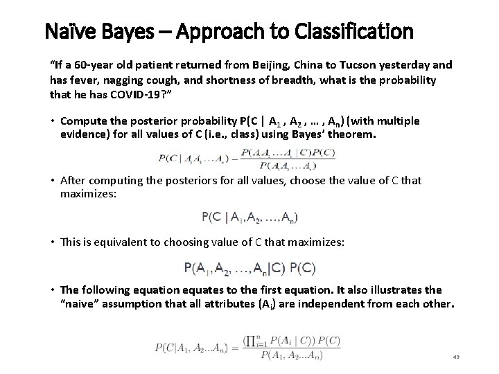
Naïve Bayes – Approach to Classification “If a 60 -year old patient returned from Beijing, China to Tucson yesterday and has fever, nagging cough, and shortness of breadth, what is the probability that he has COVID-19? ” • Compute the posterior probability P(C | A 1 , A 2 , … , An) (with multiple evidence) for all values of C (i. e. , class) using Bayes’ theorem. • After computing the posteriors for all values, choose the value of C that maximizes: • This is equivalent to choosing value of C that maximizes: • The following equation equates to the first equation. It also illustrates the “naive” assumption that all attributes (Ai) are independent from each other. 49

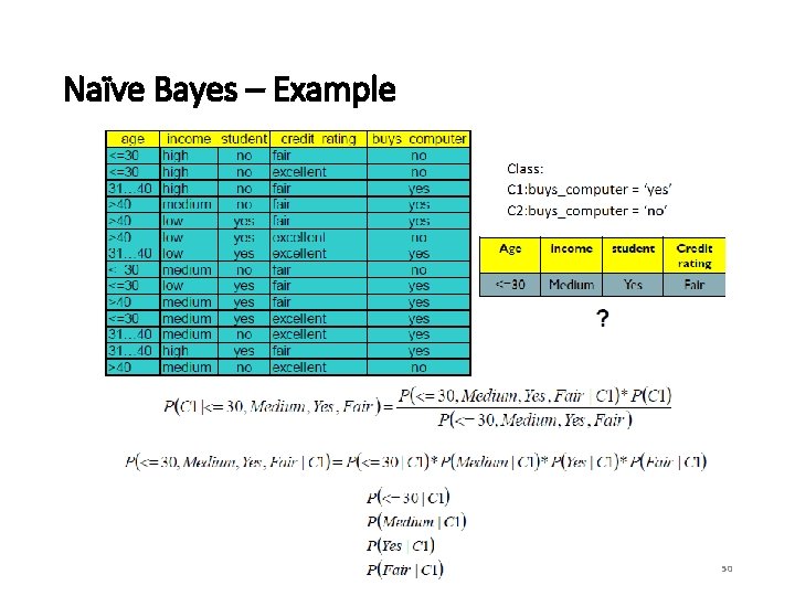
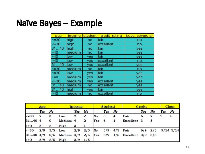
Naïve Bayes – Example 50

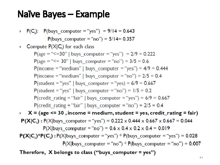
Naïve Bayes – Example 51

Naïve Bayes – Example 52

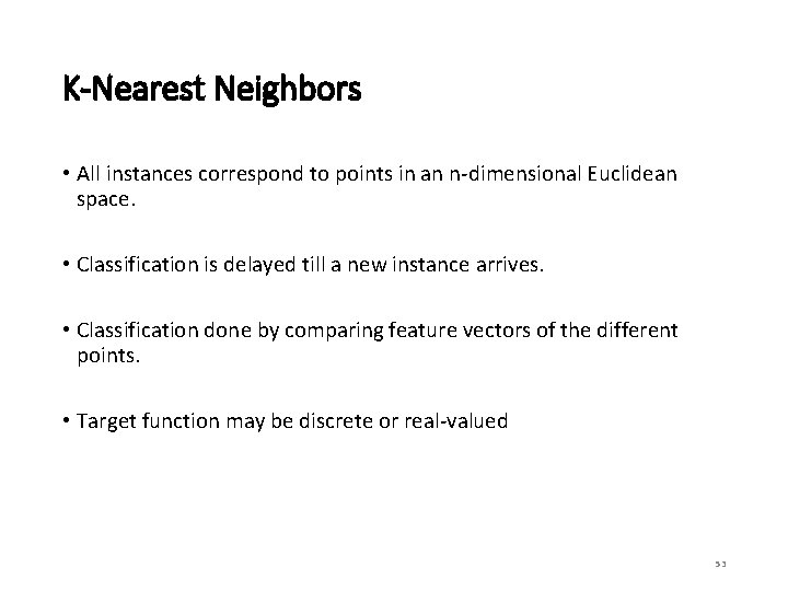
K-Nearest Neighbors • All instances correspond to points in an n-dimensional Euclidean space. • Classification is delayed till a new instance arrives. • Classification done by comparing feature vectors of the different points. • Target function may be discrete or real-valued 53

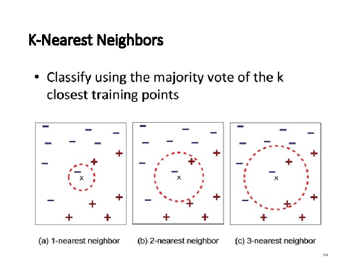
K-Nearest Neighbors 54

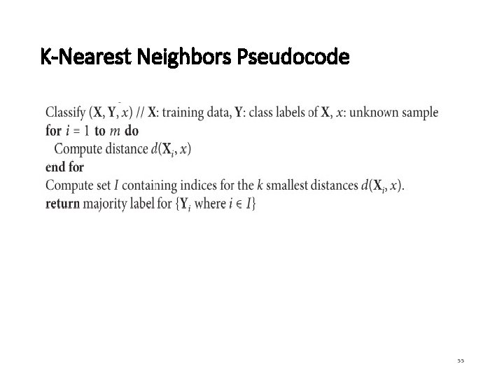
K-Nearest Neighbors Pseudocode 55

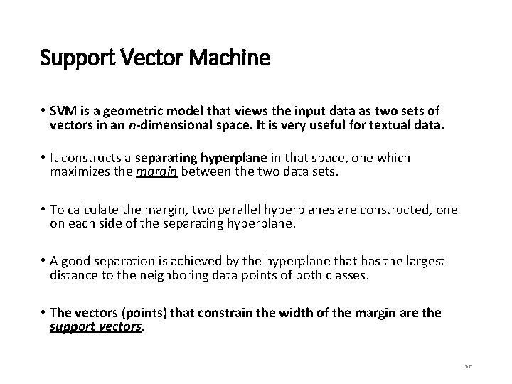
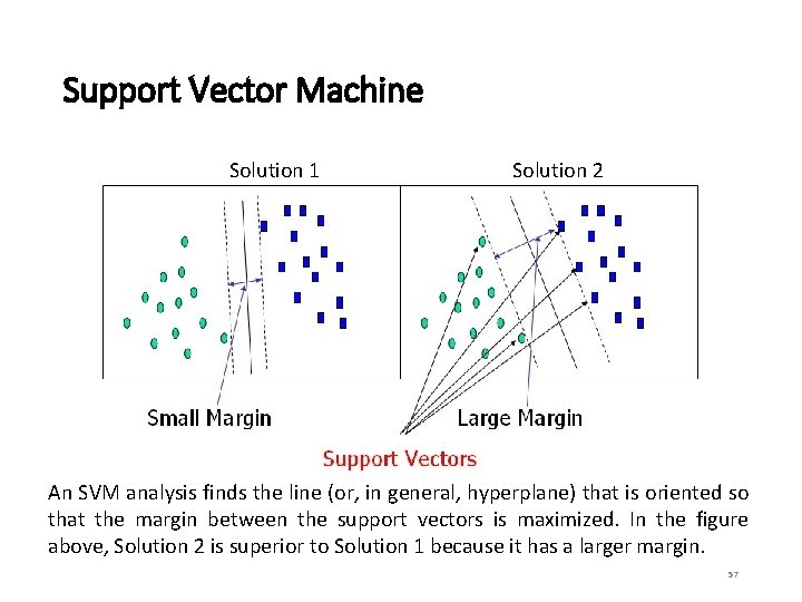
Support Vector Machine • SVM is a geometric model that views the input data as two sets of vectors in an n-dimensional space. It is very useful for textual data. • It constructs a separating hyperplane in that space, one which maximizes the margin between the two data sets. • To calculate the margin, two parallel hyperplanes are constructed, one on each side of the separating hyperplane. • A good separation is achieved by the hyperplane that has the largest distance to the neighboring data points of both classes. • The vectors (points) that constrain the width of the margin are the support vectors. 56

Support Vector Machine Solution 1 Solution 2 An SVM analysis finds the line (or, in general, hyperplane) that is oriented so that the margin between the support vectors is maximized. In the figure above, Solution 2 is superior to Solution 1 because it has a larger margin. 57

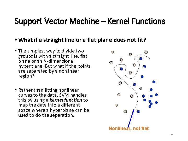
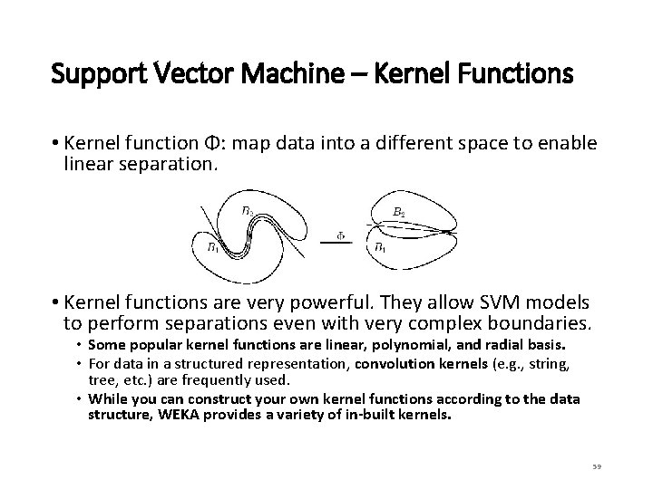
Support Vector Machine – Kernel Functions • What if a straight line or a flat plane does not fit? • The simplest way to divide two groups is with a straight line, flat plane or an N-dimensional hyperplane. But what if the points are separated by a nonlinear region? • Rather than fitting nonlinear curves to the data, SVM handles this by using a kernel function to map the data into a different space where a hyperplane can be used to do the separation. Nonlinear, not flat 58

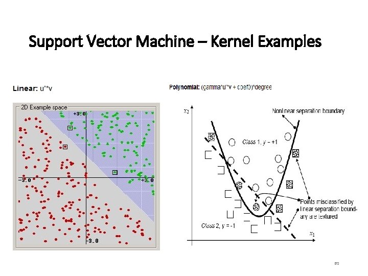
Support Vector Machine – Kernel Functions • Kernel function Φ: map data into a different space to enable linear separation. • Kernel functions are very powerful. They allow SVM models to perform separations even with very complex boundaries. • Some popular kernel functions are linear, polynomial, and radial basis. • For data in a structured representation, convolution kernels (e. g. , string, tree, etc. ) are frequently used. • While you can construct your own kernel functions according to the data structure, WEKA provides a variety of in-built kernels. 59

Support Vector Machine – Kernel Examples 60

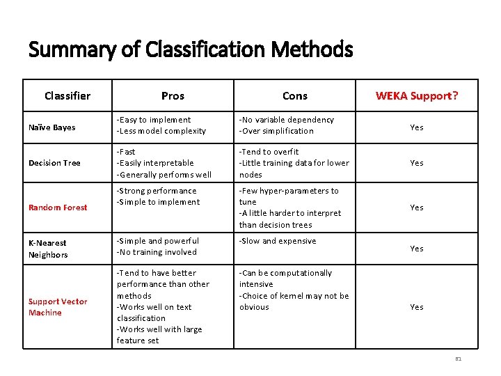
Summary of Classification Methods Classifier Pros Cons WEKA Support? Naïve Bayes -Easy to implement -Less model complexity -No variable dependency -Over simplification Yes Decision Tree -Fast -Easily interpretable -Generally performs well -Tend to overfit -Little training data for lower nodes Yes -Strong performance -Simple to implement -Few hyper-parameters to tune -A little harder to interpret than decision trees Yes K-Nearest Neighbors -Simple and powerful -No training involved -Slow and expensive Support Vector Machine -Tend to have better performance than other methods -Works well on text classification -Works well with large feature set -Can be computationally intensive -Choice of kernel may not be obvious Random Forest Yes 61

Outline • Introduction and Motivation • Terminology • Regression • Linear regression, hypothesis testing • Multiple linear regression • Classification • • • Decision Tree Random Forest Naïve Bayes K Nearest Neighbor Support Vector Machine • Evaluation metrics • Conclusion and Resources 62

Evaluation – Model Training • While the parameters of each model may differ, there are several methods to train a model. • We want to avoid overfitting a model and maximize its predictive power. • There are two standard methods for training a model: • Hold-out – reserve 2/3 of data for training and 1/3 for testing • Cross-Validation – partition data into k disjoint subsets, train on k-1 partitions, test on remaining & run k times to get average, e. g. , 10 -fold validation is commonly used. • Many software (e. g. , WEKA, Rapid. Miner) will do these methods automatically for you. 63

Evaluation • There are several questions we should ask after model training: • How predictive is the model we learned? • How reliable and accurate are the predicted results? • Which model performs better? • We want our model to perform well on our training set but also have strong predictive power. • Fortunately, various metrics applied on the testing set can help us choose the “best” model for our application. 64

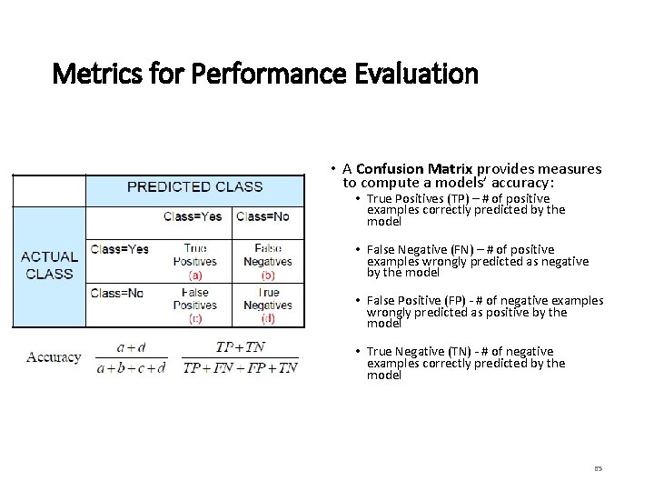
Metrics for Performance Evaluation • A Confusion Matrix provides measures to compute a models’ accuracy: • True Positives (TP) – # of positive examples correctly predicted by the model • False Negative (FN) – # of positive examples wrongly predicted as negative by the model • False Positive (FP) - # of negative examples wrongly predicted as positive by the model • True Negative (TN) - # of negative examples correctly predicted by the model 65

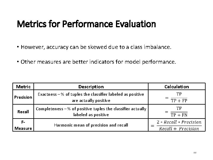
Metrics for Performance Evaluation • However, accuracy can be skewed due to a class imbalance. • Other measures are better indicators for model performance. Metric Description Precision Exactness – % of tuples the classifier labeled as positive are actually positive Recall Completeness – % of positive tuples the classifier actually labeled as positive FMeasure Harmonic mean of precision and recall Calculation 66

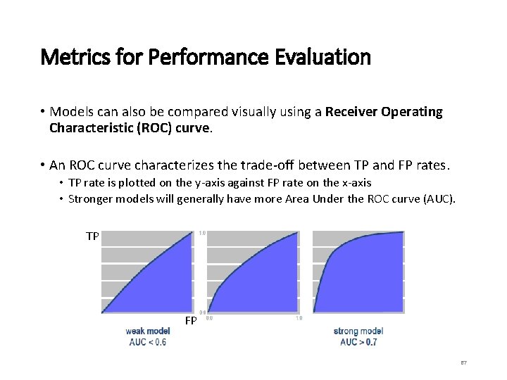
Metrics for Performance Evaluation • Models can also be compared visually using a Receiver Operating Characteristic (ROC) curve. • An ROC curve characterizes the trade-off between TP and FP rates. • TP rate is plotted on the y-axis against FP rate on the x-axis • Stronger models will generally have more Area Under the ROC curve (AUC). TP FP 67

Outline • Introduction and Motivation • Terminology • Regression • Linear regression, hypothesis testing • Multiple linear regression • Classification • • • Decision Tree Random Forest Naïve Bayes K Nearest Neighbor Support Vector Machine • Evaluation metrics • Conclusion and Resources 68

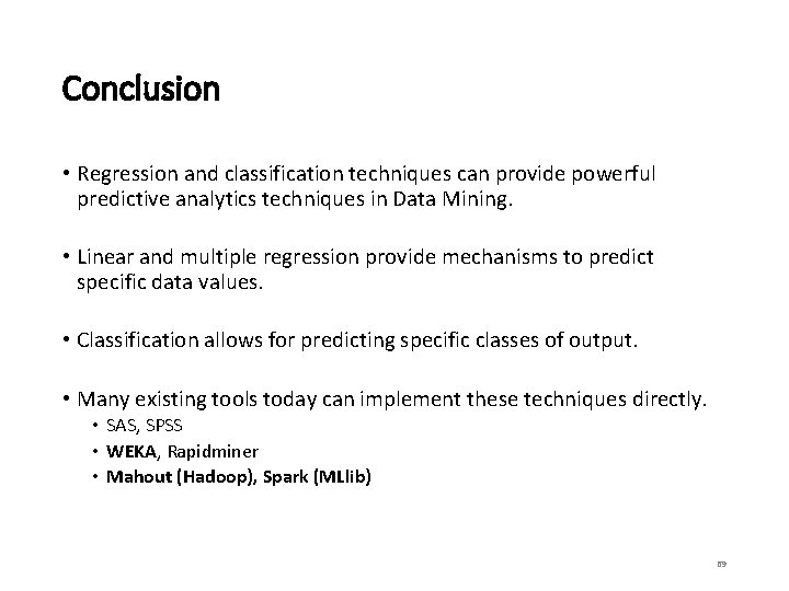
Conclusion • Regression and classification techniques can provide powerful predictive analytics techniques in Data Mining. • Linear and multiple regression provide mechanisms to predict specific data values. • Classification allows for predicting specific classes of output. • Many existing tools today can implement these techniques directly. • SAS, SPSS • WEKA, Rapidminer • Mahout (Hadoop), Spark (MLlib) 69

References Data Mining: Concepts and Techniques, 3 rd Edition. Jiawei. Han, Micheline Kamberand Jian Pei. Morgan Kaufmann Introduction to Data Mining. Pang-Ning Tan, Michael Steinbach and Vipin Kumar. Addison-Wesley Tay, B. , Hyun, J. K. , & Oh, S. (2014). A machine learning approach for specification of spinal cord injuries using fractional anisotropy values obtained from diffusion tensor images. Computational and mathematical methods in medicine, 2014. 70

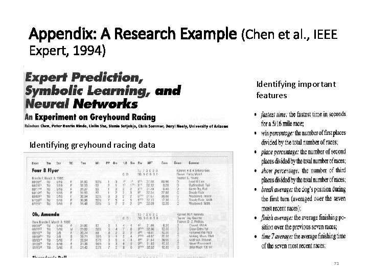
Appendix: A Research Example (Chen et al. , IEEE Expert, 1994) Identifying important features Identifying greyhound racing data 71

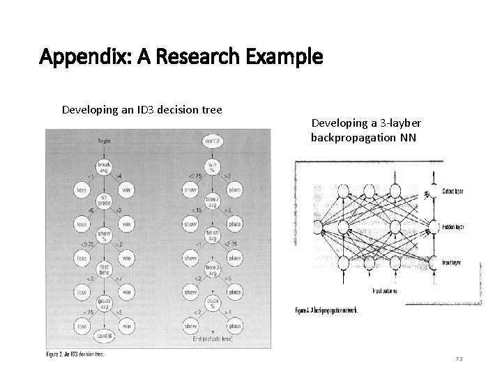
Appendix: A Research Example Developing an ID 3 decision tree Developing a 3 -layber backpropagation NN 72

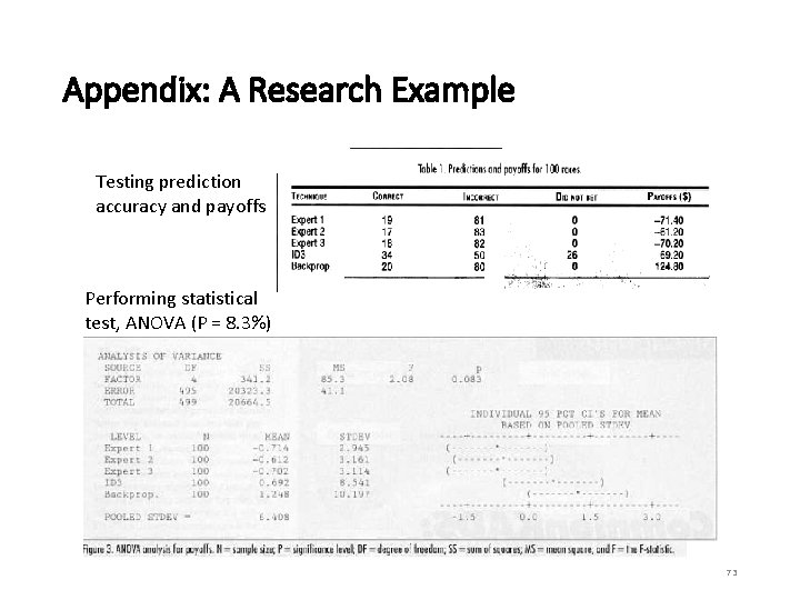
Appendix: A Research Example Testing prediction accuracy and payoffs Performing statistical test, ANOVA (P = 8. 3%) 73