Prediction Systems With Data Assimilation For Coupled Ocean


 Acoustics – Backscatter (Zooplankton) Almeira-Oran front in")
![Coupled Interdisciplinary Error Covariances x = [x. A x. O x. B] Physics: x.](https://slidetodoc.com/presentation_image/c9763ac0f6a7525ccee3f0d6721c85d7/image-8.jpg "Coupled Interdisciplinary Error Covariances x = [x. A x. O x. B] Physics: x.")


 Models and Outputs PHYSICAL MODELS • Non-hydrostatic models (PDE, x, y, z,")


 • Acoustical model uncertainties – Sound-speed")
 • Sonar system model and signal")

 1. Direct Insertion,")

![Coupled discrete state vector x (from continuous i) x = [x. A x. O]](https://slidetodoc.com/presentation_image/c9763ac0f6a7525ccee3f0d6721c85d7/image-25.jpg "Coupled discrete state vector x (from continuous i) x = [x. A x. O]")


, overlaid on bathymetry.")

 using SIRE-PDF Systems-based PDF (incorporates environmental and")


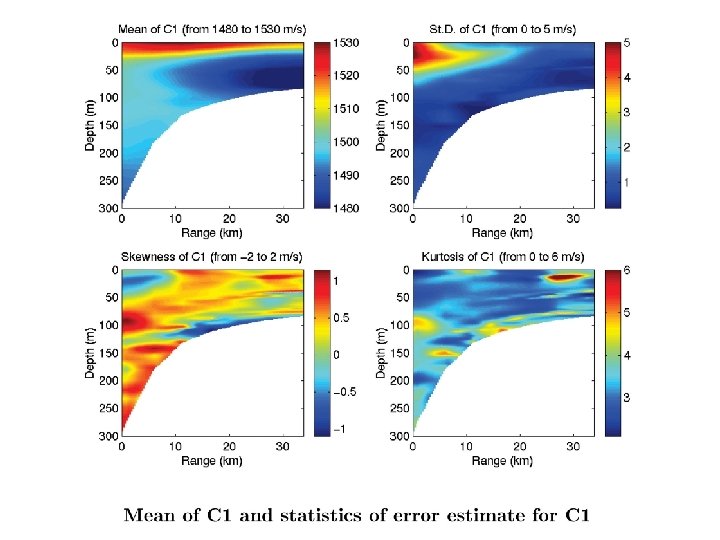
 Coupled ESSE data assimilation of sound-speed and TL data for a joint estimate")


- Slides: 52
Prediction Systems With Data Assimilation For Coupled Ocean Science And Ocean Acoustics Allan R. Robinson Pierre F. J. Lermusiaux Division of Engineering and Applied Sciences Department of Earth and Planetary Sciences Harvard University ICTCA – Honolulu, Hawaii - 11 August 2003 http: //www. deas. harvard. edu/~robinson http: //www. deas. harvard. edu/~pierrel
Prediction Systems With Data Assimilation For Coupled Ocean Science And Ocean Acoustics • Introduction • An End-to-End System: Physical-Geological. Acoustical-Signal Processing-Sonar System • Interdisciplinary Data Assimilation • An End-to-End Example – Shelfbreak PRIMER • Concluding Remarks Collaborators: Phillip Abbot (OASIS, Inc. ), Ching-Sang Chiu (NPS, Monterey), Wayne Leslie and Pat Haley (Harvard)
Interdisciplinary Ocean Science Today • Research underway on coupled physical, biological, chemical, sedimentological, acoustical, optical processes • Ocean prediction for science and operational applications has now been initiated on basin and regional scales • Interdisciplinary processes are now known to occur on multiple interactive scales in space and time with bi-directional feedbacks
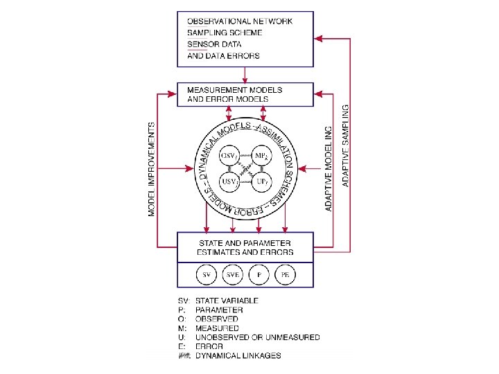
System Concept • The concept of Ocean Observing and Prediction Systems for field and parameter estimations has recently crystallized with three major components * An observational network: a suite of platforms and sensors for specific tasks * A suite of interdisciplinary dynamical models * Data assimilation schemes • Systems are modular, based on distributed information providing shareable, scalable, flexible and efficient workflow and management
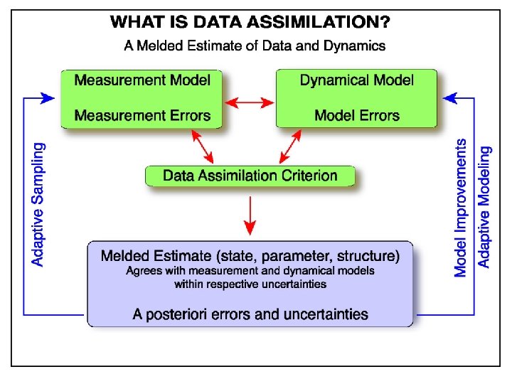
Interdisciplinary Data Assimilation • Data assimilation can contribute powerfully to understanding and modeling physicalacoustical-biological processes and is essential for ocean field prediction and parameter estimation • Model-model, data-data and data-model compatibilities are essential and dedicated interdisciplinary research is needed
Physics - Density Biology – Fluorescence (Phytoplankton) Acoustics – Backscatter (Zooplankton) Almeira-Oran front in Mediterranean Sea Fielding et al, JMS, 2001 Griffiths et al, Vol 12, THE SEA
Coupled Interdisciplinary Error Covariances x = [x. A x. O x. B] Physics: x. O = [T, S, U, V, W] Biology: x. B = [Ni, Pi, Zi, Bi, Di, Ci] Acoustics: x. A = [Pressure (p), Phase ( )] P=e {(xˆ – x ) ( xˆ – x ) } t t T PAA PAO PAB P = POA POO POB PBA PBO PBB x. O c. O
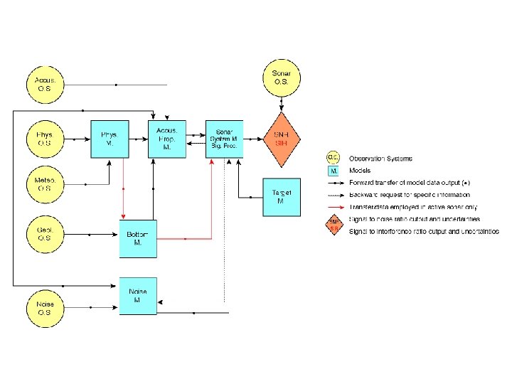
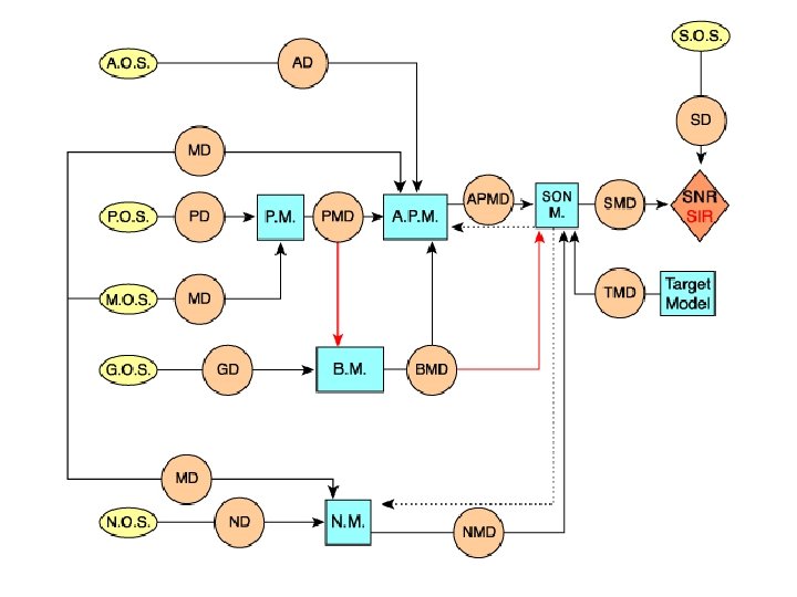
End-to-End System Concept • Sonar performance prediction requires end-to-end scientific systems: ocean physics, bottom geophysics, geo-acoustics, underwater acoustics, sonar systems and signal processing • Uncertainties inherent in measurements, models, transfer of uncertainties among linked components • Resultant uncertainty in sonar performance prediction itself • Specific applications require the consideration of a variety of specific end-to-end systems
End-to-End System
AD: Acoustical Data MD: Meteorological Data PD: Physical Data GD: Geological Data ND: Noise Data SD: Sonar Data PMD: Physical Model Data BMD: Bottom Model Data NMD: Noise Model Data APMD: Acous. Prop. Model Data SMD: Sonar Model Data TMD: Target Model Data
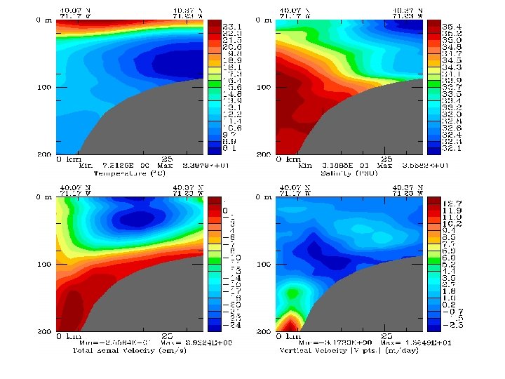
Coupled (Dynamical) Models and Outputs PHYSICAL MODELS • Non-hydrostatic models (PDE, x, y, z, t) • Primitive-Eqn. models (PDE, x, y, z, t) • Quasi-geostrophic models, shallow-water • Objective maps, balance eqn. (thermal-wind) • Feature models OUTPUTS • T, S , velocity fields and parameters, C field • Dynamical balances ACOUS. PROP. MODELS • Parabolic-Eqn. models (x, y, z, t/f) • (Coupled)-Normal-Mode parabolic-eqn. (x, z, f) • Wave number eqn. models (x, z, f: OASIS) • Ray-tracing models (CASS) OUTPUTS • Full-field TL (pressure p, phase ) • Modal decomposition of p field • Processed series: arrival strut. , travel times, etc. • CW / Broadband TL REVERBERATION MODELS (active) • Surface, volume and bottom scattering models OUTPUTS: scattering strengths BOTTOM MODELS • Hamilton model, Sediment flux models (G&G), etc • Statistical/stochastic models fit-to-data OUTPUTS • Wave-speed, density and attenuation coefficients NOISE MODELS • Wenz diagram, empirical models/rule of thumbs OUTPUTS • f-dependent ambient noise (f, x, y, z, t): due to seasurface, shipping, biologics SONAR SYS. MODELS AND SIGNAL PROCES. • Sonar equations (f, t) • Detection, localization, classification and tracking models and their inversions OUTPUTS • SNR, SIR, SE, FOM • Beamforming, spectral analyses outputs (time/frequency domains) TARGET MODELS • Measured/Empirical OUTPUTS: SL, TS for active
DEFINITION AND REPRESENTATION OF UNCERTAINTY • x = estimate of some quantity (measured, predicted, calculated) • x t = actual value (unknown true nature) • e =x- xt (unknown error) Uncertainty in x is a representation of the error estimate e e. g. probability distribution function of e • Variability in x x vs. Uncertainty in • Uncertainties in general have structures, in time and in space
MAIN SOURCES OF UNCERTAINTIES IN END-TO-END COMPONENTS • Physical model uncertainties – Bathymetry – Initial conditions – BCs: surface atmospheric, coastal-estuary and open-boundary fluxes – Parameterized processes: sub-grid-scales, turbulence closures, un-resolved processes • e. g. tides and internal tides, internal waves and solitons, microstructure and turbulence – Numerical errors: steep topographies/pressure gradient, non-convergence • Bottom/geoacoustic model uncertainties – Model structures themselves: parameterizations, variability vs. uncertainty – Measured or empirically-fit model parameters – BCs (bathymetry, bottom roughness) and initial conditions (for flux models) – 3 -D effects, non-linearities – Numerical errors: e. g. geological layer discretizations, interpolations
MAIN SOURCES OF UNCERTAINTIES IN END-TO-END COMPONENTS (Continued) • Acoustical model uncertainties – Sound-speed field (c) – Bathymetry, bottom geoacoustic attributes – BCs: Bottom roughness, sea-surface state – Scattering (volume, bottom, surface) – 3 -D effects, non-linear wave effects (non-Helmholz) – Numerical errors: e. g. c-interpolation, normal-mode at short range – Computation of broadband TL
MAIN SOURCES OF UNCERTAINTIES IN END-TO-END COMPONENTS (Continued) • Sonar system model and signal processing uncertainties – Terms in equation: SL, TL, N, AG, DT – Sonar equations themselves: 3 D effects, non-independences, multiplicative noise – Beamformer posterior uncertainties, Beamformer equations themselves • Noise model uncertainties – Ambiant noise: frequencies, directions, amplitudes, types (manmade, natural) – Measured or empirically-fit model parameters (Wenz, 1962) • Target model uncertainties – Source level, target strength (measured or empirically-fit model parameters) • Reverberation model uncertainties (active) – Scattering models themselves: parameterizations (bottom scattering, bubbles, etc) – Measured or empirically-fit model parameters
Data Assimilation
CLASSES OF DATA ASSIMILATION SCHEMES • Estimation Theory (Filtering and Smoothing) 1. Direct Insertion, Blending, Nudging 2. Optimal interpolation 3. Kalman filter/smoother 4. Bayesian estimation (Fokker-Plank equations) 5. Ensemble/Monte-Carlo methods 6. Error-subspace/Reduced-order methods: Square-root filters, e. g. SEEK 7. Error Subspace Statistical Estimation (ESSE): 5 and 6 - Lin. , LS - Linear, LS - Non-linear, Non-LS - Non-linear, LS/Non-LS - (Non)-Linear, LS -Non-linear, LS/Non-LS • Control Theory/Calculus of Variations (Smoothing) 1. “Adjoint methods” (+ descent) 2. Generalized inverse (e. g. Representer method + descent) - Lin, LS • Optimization Theory (Direct local/global smoothing) 1. Descent methods (Conjugate gradient, Quasi-Newton, etc) - Lin, LS/Non-LS 2. Simulated annealing, Genetic algorithms - Non-linear, LS/Non-LS • Hybrid Schemes • Combinations of the above
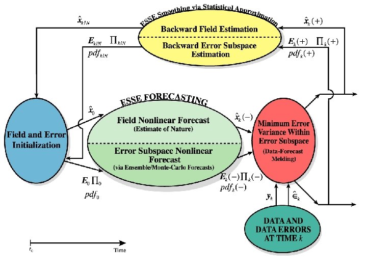
Harvard Ocean Prediction System - HOPS
Coupled discrete state vector x (from continuous i) x = [x. A x. O] Physics: x. O = [T, S, U, V, W] Acoustics: x. A = [Pressure (p), Phase ( )] Coupled error covariance P=e {(xˆ – x ) ( xˆ – x ) } t t T P= Coupled assimilation x+ = x- + PHT [HPHT+R]-1 (y-Hx-); x- = A priori estimate (for forecast) x+ = A posteriori estimate (after assimilation) PAA PAO POA POO c. O
Real-Time Initialization of the Dominant Error Covariance Decomposition • Real-time Assumptions • Dominant uncertainties are missing or uncertain variability in initial state, e. g. , smaller mesoscale variability • Issues • Some state variables are not observed • Uncertain variability is multiscale • Approach: Multi-variate, 3 D, Multi-scale • “Observed” portions • Directly specified and eigendecomposed from differences between the intial state and data, and/or from a statistical model fit to these differences • “Non-observed” portions • Keep “observed” portions fixed and compute “nonobserved”portions from ensemble of numerical (stochastic) dynamical simulations
PRIMER
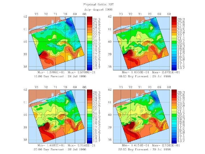
PRIMER End-to-End Problem Initial Focus on Passive Sonar Problem Location: Shelfbreak PRIMER Region Season: July-August 1996 Sonar System (Receiver): Passive Towed Array Target: Simulated UUV (with variable source level) Frequency Range: 100 to 500 Hz Geometries: Receiver operating on the shelf shallow water; target operating on the shelf slope (deeper water than receiver)
PHYSICAL-ACOUSTICAL FILTERING IN A SHELFBREAK ENVIRONMENT
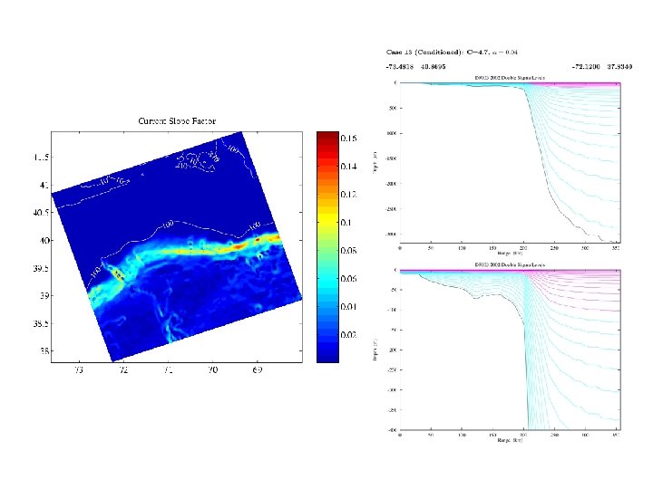
Acoustic paths considered (as in Shelfbreak-PRIMER), overlaid on bathymetry.
Histogram of Difference Between Model and Measured SIR, SIRE-PDF • Represents uncertainty in our ability to model actual performance of system • Accounts for inherent variability of environment not known by current model Difference Between Model and Measurement, d. B
Determination of PPD (Predictive Probability Of Detection) using SIRE-PDF Systems-based PDF (incorporates environmental and system uncertainty) Used by UNITES to characterize and transfer uncertainty from environment through end-to-end problems
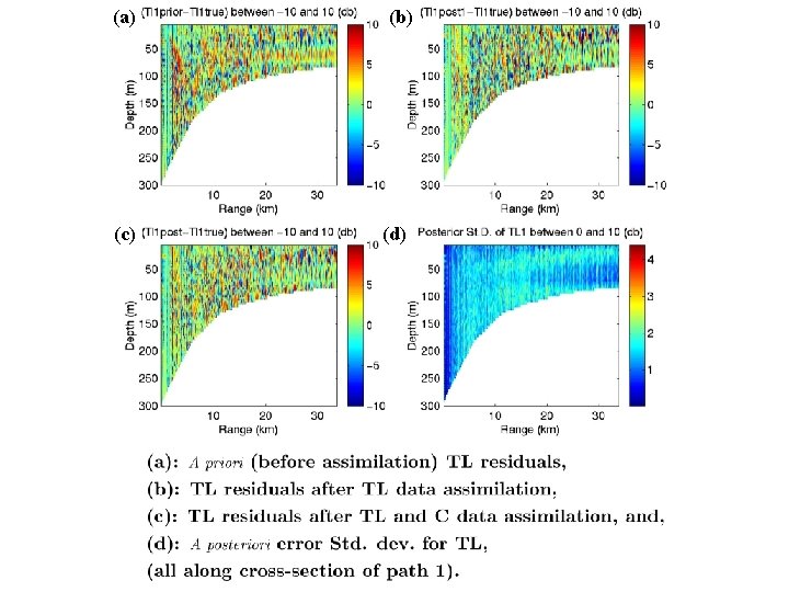
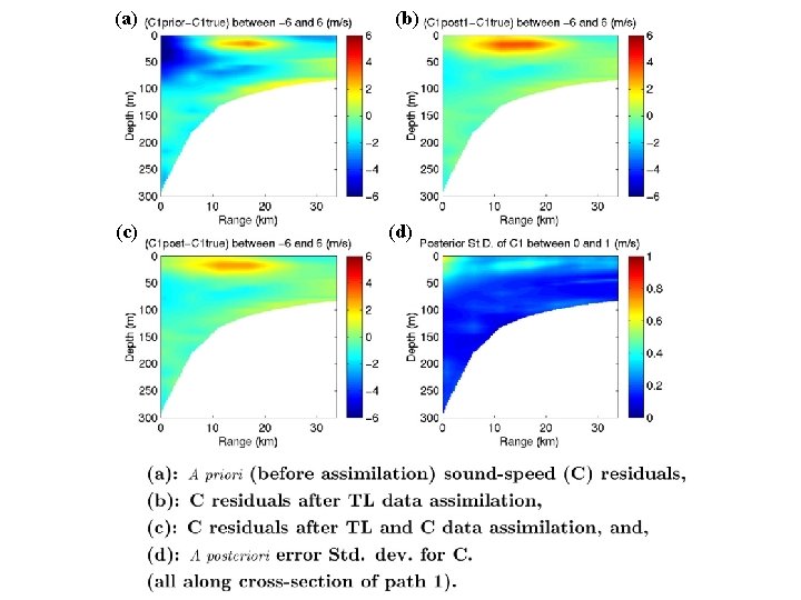
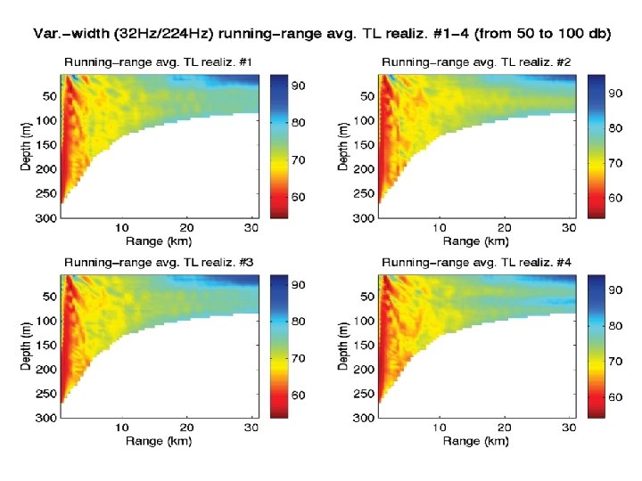
Starting with physical environmental data, compute the PPD from first principals via broadband TL • Novel approach: coupled physical-acoustical data assimilation method is used in TL estimation • Methodology: coupled physical-acoustical identicaltwin experiment – ESSE based – Model generates “true” ocean – 79 member ensemble for a priori estimate – Coarsely sampled CTD and TL measurements are assimilated for a posteriori estimate
Monte Carlo simulation example: transfer of ocean physical forecast Uncertainty to acoustic prediction uncertainty in a shelfbreak environment.
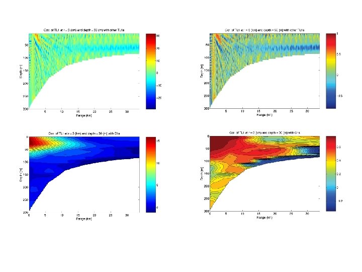
(a) Coupled ESSE data assimilation of sound-speed and TL data for a joint estimate of sound -speed and TL fields (c) (b) (d)
Predicted PDF of broadband TL
PDF of broadband TL after assimilation
CONCLUSIONS: Coupled ESSE Identical-Twin Experiments • Oceans physics/acoustics data assimilation: carried-out as a single multi-scale joint estimation for the first time, using higher-moments to characterize uncertainties • ESSE nonlinear coupled assimilation recovers fine-scale TL structures (10 -100 m) and mesoscale ocean physics (10 km) from coarse TL data (towed-receiver at 70 m depth, one data every 500 m) and/or coarse C data (2 -3 profiles over 40 km) • Two notable coupled processes: – Shoreward meander of upper-front leads to less loss in acoustic waveguide (cold pool) on shelf – Corresponding thickening of thermocline at the front induces phase shifts in ray patterns on the shelf • Broadband TL uncertainties predicted to be range and depth dependent • Coupled DA sharpens and homogenizes broadband PDFs
Summary
End-to-End System Concept • Sonar performance prediction requires end-to-end scientific systems: ocean physics, bottom geophysics, geo-acoustics, underwater acoustics, sonar systems and signal processing • Uncertainties inherent in measurements, models, transfer of uncertainties among linked components • Resultant uncertainty in sonar performance prediction itself • Specific applications require the consideration of a variety of specific end-to-end systems
Representation of Uncertainties • Research on the representation of uncertainties and transfers is important • Efficient representations vary with scales, processes and applications • Attribution of uncertainties to unmeasured or unmeasurable variabilities, data errors, model errors, and methodological errors • Sensitivity studies to determine the hierarchy of uncertainties • Representation of uncertainties via PDFs is yielding useful results o research on nonlinear and non-Gaussian effects o construction of multivariate interdisciplinary PDFs • Confidence level of the uncertainty should be estimated for scientific purposes • Monte-Carlo (ensemble) is a general method for transferring uncertainties across interfaces o results used to develop useful representations in terms of scalars, vectors, covariances, etc.
Data Assimilation • Data assimilation in physical oceanography is now being extended to interdisciplinary ocean science • Data and models are melded to estimate state variables (fields) and parameters estimation theory or control theory techniques o melded estimate better than either the model or the data. o weighting scheme based on data errors and model errors o data assimilation based on errors is naturally applicable to uncertainty studies o
Data Assimilation • Assimilation of physical data extends the usefulness of that data for acoustic propagation • Data assimilation coupling oceanography and acoustics is being initiated assimilation of transmission loss, noise and reverberation o research will involve PDFs which are range, depth and azimuth dependent o • Multivariate approach, using interdisciplinary acoustical-physicalgeological covariance matrices, is a key element of the method.
CONCLUSIONS • Entering a new era of fully interdisciplinary ocean science and ocean acoustics • Ocean prediction systems for science, operations and management • Interdisciplinary estimation of state variables and error fields via multivariate physicalbiological-acoustical data assimilation • Novel and challenging opportunities for theoretical and computational acoustics