Prediction and Search in Probabilistic Worlds Markov Systems

Prediction and Search in Probabilistic Worlds Markov Systems, Markov Decision Processes, and Dynamic Programming Note to other teachers and users of these slides. Andrew would be delighted if you found this source material useful in giving your own lectures. Feel free to use these slides verbatim, or to modify them to fit your own needs. Power. Point originals are available. If you make use of a significant portion of these slides in your own lecture, please include this message, or the following link to the source repository of Andrew’s tutorials: http: //www. cs. cmu. edu/~awm/tutorials. Comments and corrections gratefully received. Andrew W. Moore Professor School of Computer Science Carnegie Mellon University www. cs. cmu. edu/~awm awm@cs. cmu. edu 412 -268 -7599 Copyright © 2002, 2004, Andrew W. Moore April 21 st, 2002

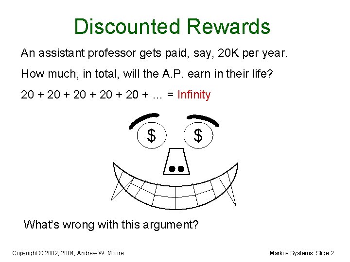
Discounted Rewards An assistant professor gets paid, say, 20 K per year. How much, in total, will the A. P. earn in their life? 20 + 20 + … = Infinity $ $ What’s wrong with this argument? Copyright © 2002, 2004, Andrew W. Moore Markov Systems: Slide 2

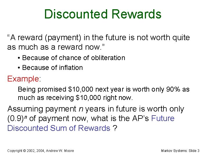
Discounted Rewards “A reward (payment) in the future is not worth quite as much as a reward now. ” • Because of chance of obliteration • Because of inflation Example: Being promised $10, 000 next year is worth only 90% as much as receiving $10, 000 right now. Assuming payment n years in future is worth only (0. 9)n of payment now, what is the AP’s Future Discounted Sum of Rewards ? Copyright © 2002, 2004, Andrew W. Moore Markov Systems: Slide 3

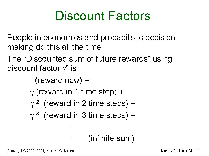
Discount Factors People in economics and probabilistic decisionmaking do this all the time. The “Discounted sum of future rewards” using discount factor g” is (reward now) + g (reward in 1 time step) + g 2 (reward in 2 time steps) + g 3 (reward in 3 time steps) + : : (infinite sum) Copyright © 2002, 2004, Andrew W. Moore Markov Systems: Slide 4

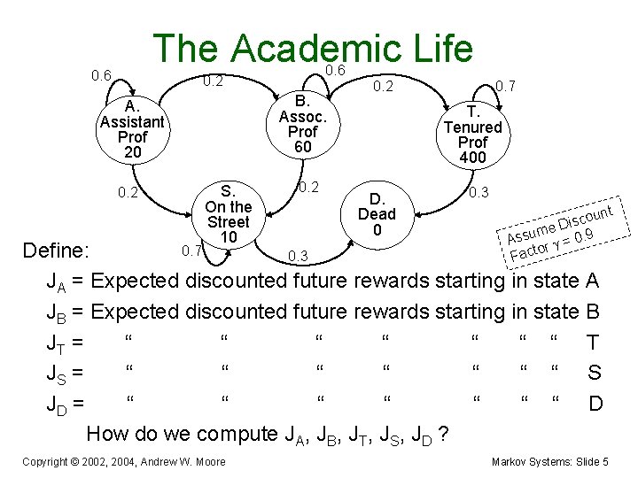
The Academic Life 0. 6 0. 2 B. Assoc. Prof 60 A. Assistant Prof 20 0. 2 S. On the Street 10 0. 2 0. 7 T. Tenured Prof 400 D. Dead 0 0. 3 ount c s i me D 0. 9 u s s A rg= o t c Fa 0. 7 Define: 0. 3 JA = Expected discounted future rewards starting in state A JB = Expected discounted future rewards starting in state B JT = “ “ “ “ T JS = “ “ “ “ S JD = “ “ “ “ D How do we compute JA, JB, JT, JS, JD ? Copyright © 2002, 2004, Andrew W. Moore Markov Systems: Slide 5

Computing the Future Rewards of an Academic Copyright © 2002, 2004, Andrew W. Moore

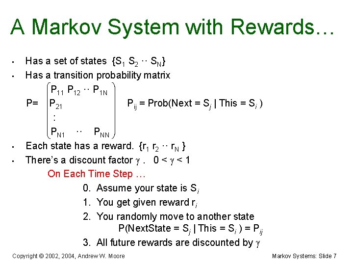
A Markov System with Rewards… • • Has a set of states {S 1 S 2 ·· SN} Has a transition probability matrix P 11 P 12 ·· P 1 N P= P 21 Pij = Prob(Next = Sj | This = Si ) : PN 1 ·· PNN Each state has a reward. {r 1 r 2 ·· r. N } There’s a discount factor g. 0 < g < 1 On Each Time Step … 0. Assume your state is Si 1. You get given reward ri 2. You randomly move to another state P(Next. State = Sj | This = Si ) = Pij 3. All future rewards are discounted by g Copyright © 2002, 2004, Andrew W. Moore Markov Systems: Slide 7

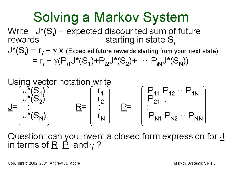
Solving a Markov System Write J*(Si) = expected discounted sum of future rewards starting in state Si J*(Si) = ri + g x (Expected future rewards starting from your next state) = ri + g(Pi 1 J*(S 1)+Pi 2 J*(S 2)+ ··· Pi. NJ*(SN)) Using vector notation write J*(S 1) r 1 J*(S 2) r 2 J= : R= : J*(SN) r. N P= P 11 P 12 ·· P 1 N P 21 ·. : PN 1 PN 2 ·· PNN Question: can you invent a closed form expression for J in terms of R P and g ? Copyright © 2002, 2004, Andrew W. Moore Markov Systems: Slide 8

Solving a Markov System with Matrix Inversion • • Upside: You get an exact answer Downside: If you have 100, 000 states you’re solving a 100, 000 by 100, 000 system of equations. Copyright © 2002, 2004, Andrew W. Moore Markov Systems: Slide 10

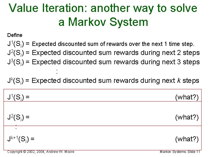
Value Iteration: another way to solve a Markov System Define J 1(Si) = Expected discounted sum of rewards over the next 1 time step. J 2(Si) = Expected discounted sum rewards during next 2 steps J 3(Si) = Expected discounted sum rewards during next 3 steps : Jk(Si) = Expected discounted sum rewards during next k steps J 1(Si) = (what? ) J 2(Si) = : (what? ) Jk+1(Si) = (what? ) Copyright © 2002, 2004, Andrew W. Moore Markov Systems: Slide 11

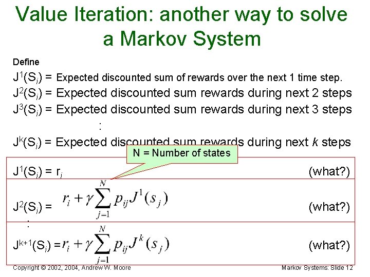
Value Iteration: another way to solve a Markov System Define J 1(Si) = Expected discounted sum of rewards over the next 1 time step. J 2(Si) = Expected discounted sum rewards during next 2 steps J 3(Si) = Expected discounted sum rewards during next 3 steps : Jk(Si) = Expected discounted sum rewards during next k steps N = Number of states J 1(Si) = ri (what? ) J 2(Si) = : (what? ) Jk+1(Si) = (what? ) Copyright © 2002, 2004, Andrew W. Moore Markov Systems: Slide 12

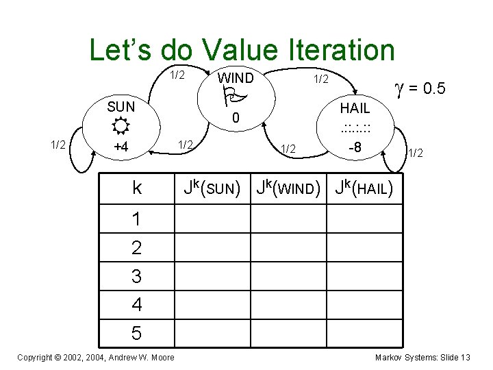
Let’s do Value Iteration 1/2 +4 k 0 1/2 g = 0. 5 1/2

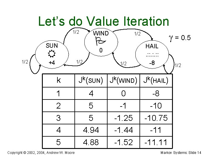
Let’s do Value Iteration 1/2 +4 k 1 2 3 4 5 Copyright © 2002, 2004, Andrew W. Moore 0 1/2 g = 0. 5 1/2 SUN WIND 1/2 HAIL. : : -8 1/2 Jk(SUN) Jk(WIND) Jk(HAIL) 4 5 5 4. 94 4. 88 0 -1 -1. 25 -1. 44 -1. 52 -8 -10. 75 -11. 11 Markov Systems: Slide 14

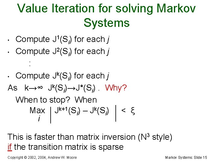
Value Iteration for solving Markov Systems Compute J 1(Si) for each j • Compute J 2(Si) for each j : • Compute Jk(Si) for each j As k→∞ Jk(Si)→J*(Si). Why? When to stop? When Max Jk+1(Si) – Jk(Si) < ξ i • This is faster than matrix inversion (N 3 style) if the transition matrix is sparse Copyright © 2002, 2004, Andrew W. Moore Markov Systems: Slide 15

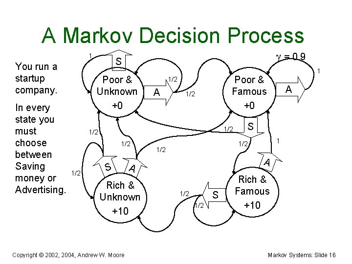
A Markov Decision Process 1 You run a startup company. In every state you must choose between Saving money or Advertising. g = 0. 9 S Poor & Unknown +0 Poor & Famous +0 1/2 A 1/2 1/2 1/2 S Copyright © 2002, 2004, Andrew W. Moore A S 1 1/2 A A Rich & Unknown +10 1 S 1/2 Rich & Famous +10 Markov Systems: Slide 16

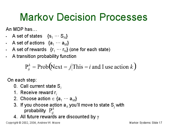
Markov Decision Processes An MDP has… • A set of states {s 1 ··· SN} • A set of actions {a 1 ··· a. M} • A set of rewards {r 1 ··· r. N} (one for each state) • A transition probability function On each step: 0. Call current state Si 1. Receive reward ri 2. Choose action {a 1 ··· a. M} 3. If you choose action ak you’ll move to state Sj with probability 4. All future rewards are discounted by g Copyright © 2002, 2004, Andrew W. Moore Markov Systems: Slide 17

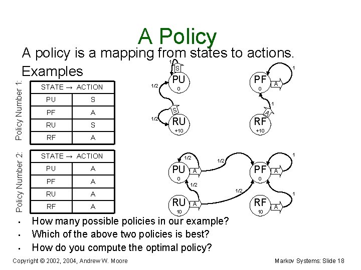
A Policy A policy is a mapping from states to actions. S Examples 1 Policy Number 2: Policy Number 1: 1 • • • STATE → ACTION PU S PF A RU S RF A 1/2 PU PF 0 0 A 1 S 1/2 A RU RF +10 STATE → ACTION 1 1/2 PU A PU PF A 0 RU A RF A 1/2 PF A A 0 1/2 RU A 10 1 RF 10 A How many possible policies in our example? Which of the above two policies is best? How do you compute the optimal policy? Copyright © 2002, 2004, Andrew W. Moore Markov Systems: Slide 18

Interesting Fact For every M. D. P. there exists an optimal policy. It’s a policy such that for every possible start state there is no better option than to follow the policy. (Not proved in this lecture) Copyright © 2002, 2004, Andrew W. Moore Markov Systems: Slide 19

Computing the Optimal Policy Idea One: Run through all possible policies. Select the best.

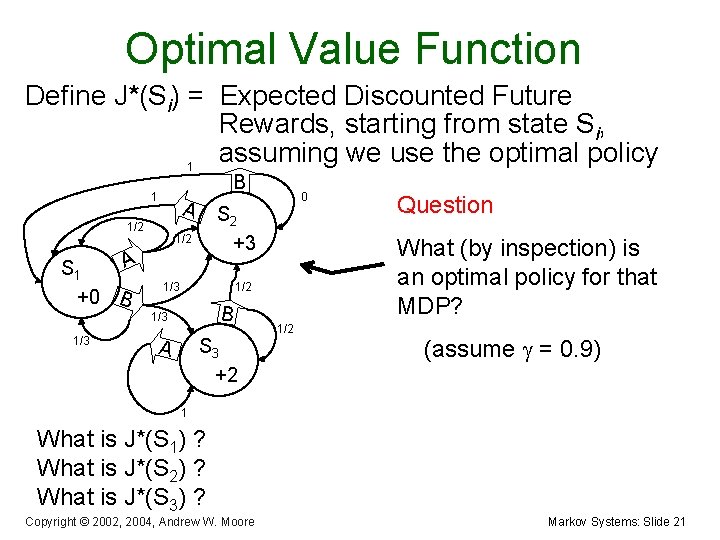
Optimal Value Function Define J*(Si) = Expected Discounted Future Rewards, starting from state Si, assuming we use the optimal policy 1 B 1 A 1/2 S 2 +3 1/2 A S 1 +0 B 1/3 B S 3 +2 A Question What (by inspection) is an optimal policy for that MDP? 1/2 1/3 0 1/2 (assume g = 0. 9) 1 What is J*(S 1) ? What is J*(S 2) ? What is J*(S 3) ? Copyright © 2002, 2004, Andrew W. Moore Markov Systems: Slide 21

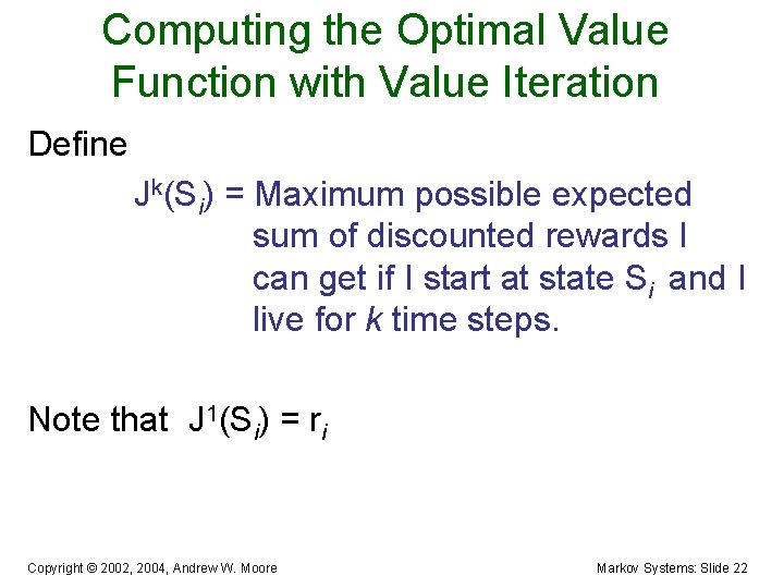
Computing the Optimal Value Function with Value Iteration Define Jk(Si) = Maximum possible expected sum of discounted rewards I can get if I start at state Si and I live for k time steps. Note that J 1(Si) = ri Copyright © 2002, 2004, Andrew W. Moore Markov Systems: Slide 22

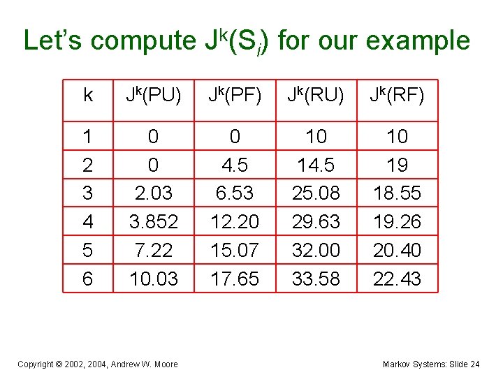
Let’s compute Jk(Si) for our example k Jk(PU) Jk(PF) Jk(RU) Jk(RF) 1 2 3 4 5 6 0 0 2. 03 3. 852 7. 22 10. 03 0 4. 5 6. 53 12. 20 15. 07 17. 65 10 14. 5 25. 08 29. 63 32. 00 33. 58 10 19 18. 55 19. 26 20. 40 22. 43 Copyright © 2002, 2004, Andrew W. Moore Markov Systems: Slide 24

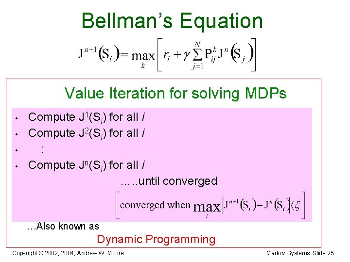
Bellman’s Equation Value Iteration for solving MDPs • • Compute J 1(Si) for all i Compute J 2(Si) for all i : Compute Jn(Si) for all i …. . until converged …Also known as Dynamic Programming Copyright © 2002, 2004, Andrew W. Moore Markov Systems: Slide 25

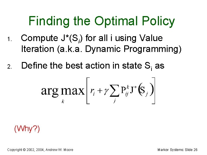
Finding the Optimal Policy 1. 2. Compute J*(Si) for all i using Value Iteration (a. k. a. Dynamic Programming) Define the best action in state Si as (Why? ) Copyright © 2002, 2004, Andrew W. Moore Markov Systems: Slide 26

Applications of MDPs This extends the search algorithms of your first lectures to the case of probabilistic next states. Many important problems are MDPs…. … Robot path planning … Travel route planning … Elevator scheduling … Bank customer retention … Autonomous aircraft navigation … Manufacturing processes … Network switching & routing Copyright © 2002, 2004, Andrew W. Moore Markov Systems: Slide 27

Asynchronous D. P. Value Iteration: “Backup S 1”, “Backup S 2”, ···· “Backup SN”, then “Backup S 1”, “Backup S 2”, ···· repeat : : There’s no reason that you need to do the backups in order! Random Order …still works. Easy to parallelize (Dyna, Sutton 91) On-Policy Order Simulate the states that the system actually visits. Efficient Order e. g. Prioritized Sweeping [Moore 93] Q-Dyna [Peng & Williams 93] Copyright © 2002, 2004, Andrew W. Moore Markov Systems: Slide 28

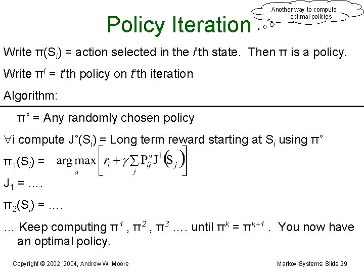
Policy Iteration Another way to compute optimal policies Write π(Si) = action selected in the i’th state. Then π is a policy. Write πt = t’th policy on t’th iteration Algorithm: π˚ = Any randomly chosen policy i compute J˚(Si) = Long term reward starting at Si using π˚ π1(Si) = J 1 = …. π2(Si) = …. … Keep computing π1 , π2 , π3 …. until πk = πk+1. You now have an optimal policy. Copyright © 2002, 2004, Andrew W. Moore Markov Systems: Slide 29

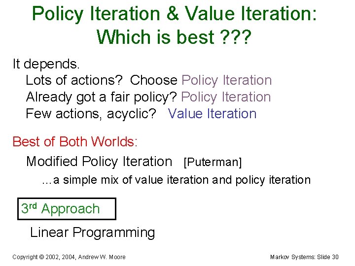
Policy Iteration & Value Iteration: Which is best ? ? ? It depends. Lots of actions? Choose Policy Iteration Already got a fair policy? Policy Iteration Few actions, acyclic? Value Iteration Best of Both Worlds: Modified Policy Iteration [Puterman] …a simple mix of value iteration and policy iteration 3 rd Approach Linear Programming Copyright © 2002, 2004, Andrew W. Moore Markov Systems: Slide 30

Time to Moan What’s the biggest problem(s) with what we’ve seen so far? Copyright

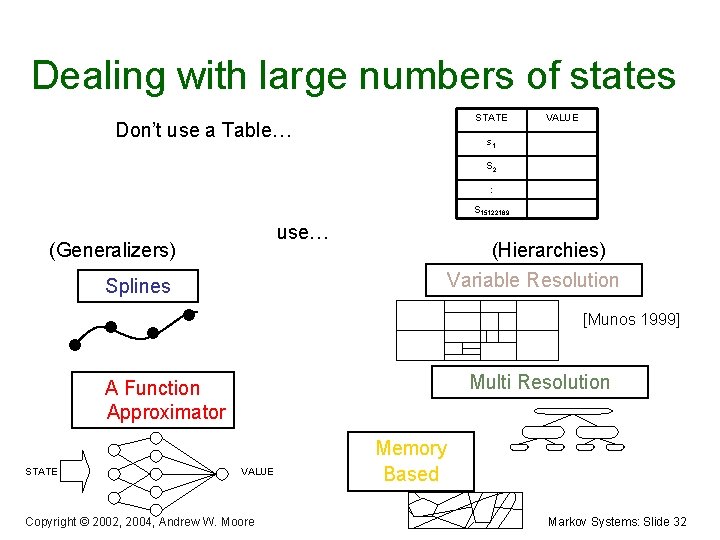
Dealing with large numbers of states STATE Don’t use a Table… VALUE s 1 S 2 : S 15122189 use… (Generalizers) (Hierarchies) Variable Resolution Splines [Munos 1999] Multi Resolution A Function Approximator STATE VALUE Copyright © 2002, 2004, Andrew W. Moore Memory Based Markov Systems: Slide 32

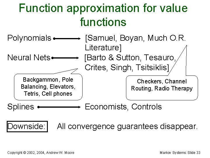
Function approximation for value functions Polynomials [Samuel, Boyan, Much O. R. Literature] [Barto & Sutton, Tesauro, Crites, Singh, Tsitsiklis] Neural Nets Backgammon, Pole Balancing, Elevators, Tetris, Cell phones Splines Downside: Checkers, Channel Routing, Radio Therapy Economists, Controls All convergence guarantees disappear. Copyright © 2002, 2004, Andrew W. Moore Markov Systems: Slide 33

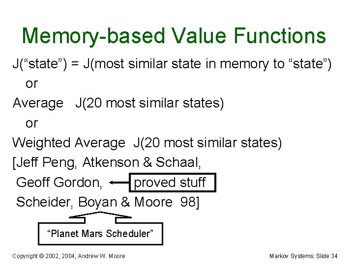
Memory-based Value Functions J(“state”) = J(most similar state in memory to “state”) or Average J(20 most similar states) or Weighted Average J(20 most similar states) [Jeff Peng, Atkenson & Schaal, Geoff Gordon, proved stuff Scheider, Boyan & Moore 98] “Planet Mars Scheduler” Copyright © 2002, 2004, Andrew W. Moore Markov Systems: Slide 34

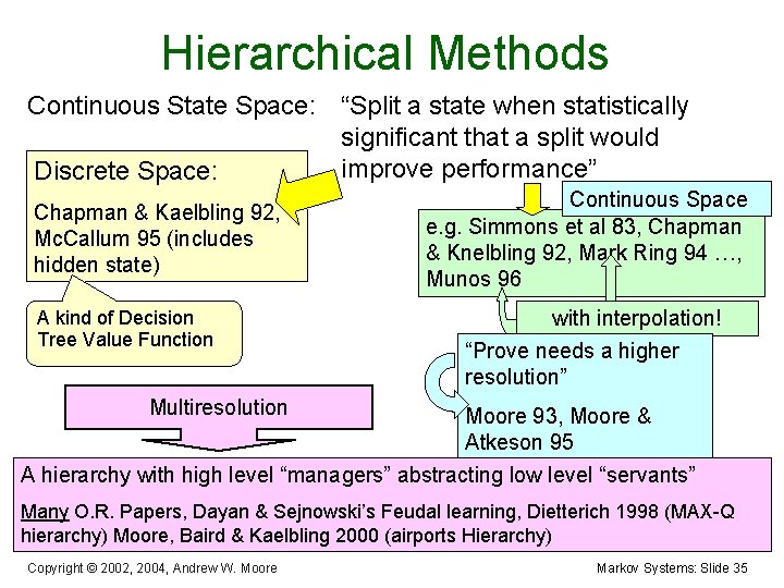
Hierarchical Methods Continuous State Space: “Split a state when statistically significant that a split would improve performance” Discrete Space: Chapman & Kaelbling 92, Mc. Callum 95 (includes hidden state) A kind of Decision Tree Value Function Continuous Space e. g. Simmons et al 83, Chapman & Knelbling 92, Mark Ring 94 …, Munos 96 with interpolation! “Prove needs a higher resolution” Multiresolution Moore 93, Moore & Atkeson 95 A hierarchy with high level “managers” abstracting low level “servants” Many O. R. Papers, Dayan & Sejnowski’s Feudal learning, Dietterich 1998 (MAX-Q hierarchy) Moore, Baird & Kaelbling 2000 (airports Hierarchy) Copyright © 2002, 2004, Andrew W. Moore Markov Systems: Slide 35

What You Should Know • • Definition of a Markov System with Discounted rewards How to solve it with Matrix Inversion How (and why) to solve it with Value Iteration Definition of an MDP, and value iteration to solve an MDP Policy iteration Great respect for the way this formalism generalizes the deterministic searching of the start of the class But awareness of what has been sacrificed. Copyright © 2002, 2004, Andrew W. Moore Markov Systems: Slide 36