Predicting Interest Rates Statistical Models Economic vs Statistical

Predicting Interest Rates Statistical Models

Economic vs. Statistical Models l Economic models are designed to match correlations between interest rates and other economic aggregate variables l Pro: Economic (structural) models use all the latest information available to predict interest rate movements l Con: They require a lot of data, the equation can be quite complex, and over longer time periods are very inaccurate

Economic vs. Statistical Models l Statistical models are designed to match the dynamics of interest rates and the yield curve using past behavior. l Pro: Statistical Models require very little data and are generally easy to calculate l Con: Statistical models rely entirely on the past. They don’t incorporate new information.

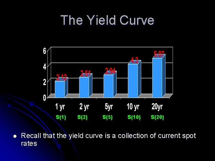
The Yield Curve S(1) l S(2) S(5) S(10) S(20) Recall that the yield curve is a collection of current spot rates

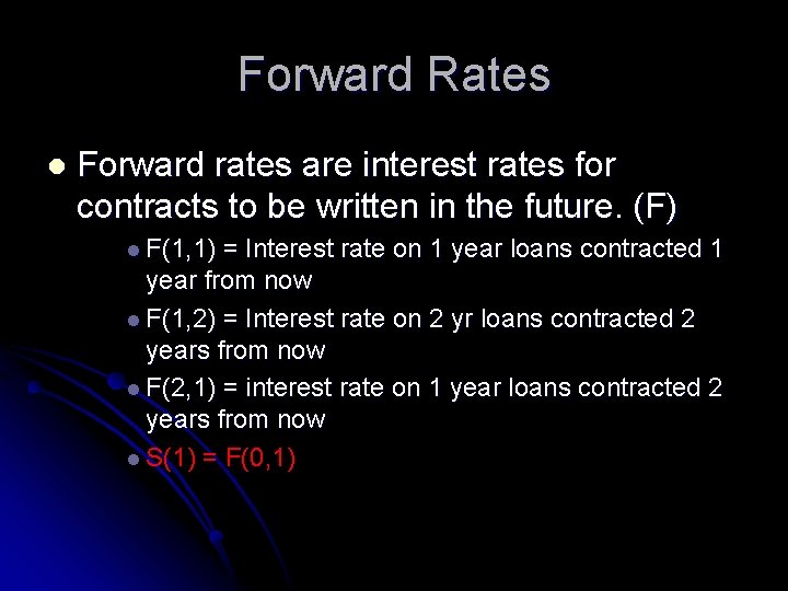
Forward Rates l Forward rates are interest rates for contracts to be written in the future. (F) l F(1, 1) = Interest rate on 1 year loans contracted 1 year from now l F(1, 2) = Interest rate on 2 yr loans contracted 2 years from now l F(2, 1) = interest rate on 1 year loans contracted 2 years from now l S(1) = F(0, 1)

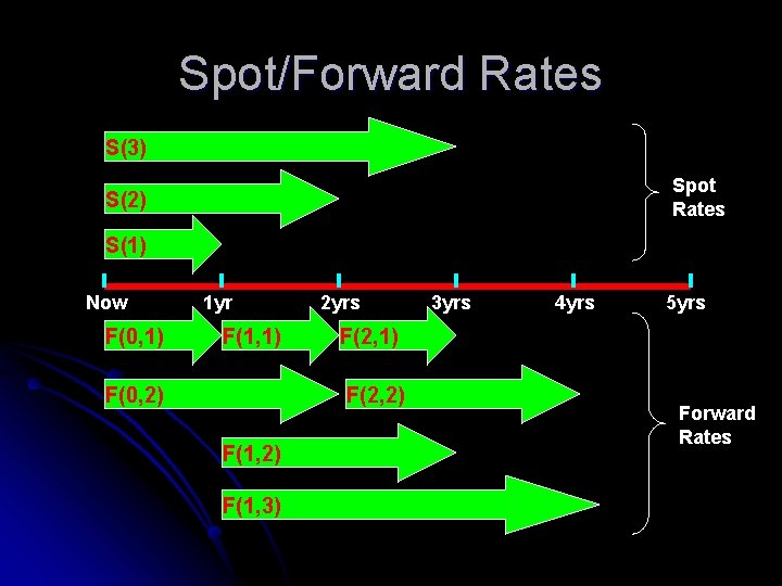
Spot/Forward Rates S(3) Spot Rates S(2) S(1) Now F(0, 1) 1 yr F(1, 1) F(0, 2) 2 yrs F(1, 3) 4 yrs 5 yrs F(2, 1) F(2, 2) F(1, 2) 3 yrs Forward Rates

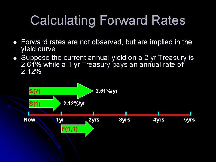
Calculating Forward Rates l l Forward rates are not observed, but are implied in the yield curve Suppose the current annual yield on a 2 yr Treasury is 2. 61% while a 1 yr Treasury pays an annual rate of 2. 12% 2. 61%/yr S(2) S(1) Now 2. 12%/yr 1 yr F(1, 1) 2 yrs 3 yrs 4 yrs 5 yrs

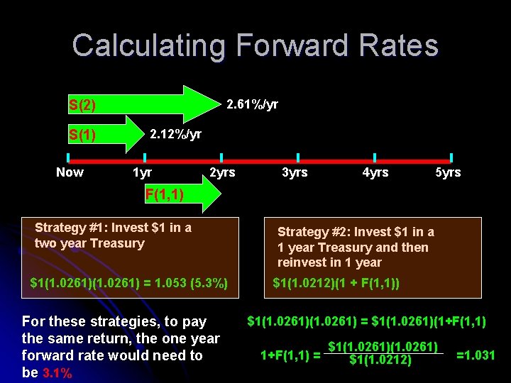
Calculating Forward Rates 2. 61%/yr S(2) S(1) Now 2. 12%/yr 1 yr 2 yrs 3 yrs 4 yrs 5 yrs F(1, 1) Strategy #1: Invest $1 in a two year Treasury $1(1. 0261) = 1. 053 (5. 3%) For these strategies, to pay the same return, the one year forward rate would need to be 3. 1% Strategy #2: Invest $1 in a 1 year Treasury and then reinvest in 1 year $1(1. 0212)(1 + F(1, 1)) $1(1. 0261) = $1(1. 0261)(1+F(1, 1) = $1(1. 0261) $1(1. 0212) =1. 031

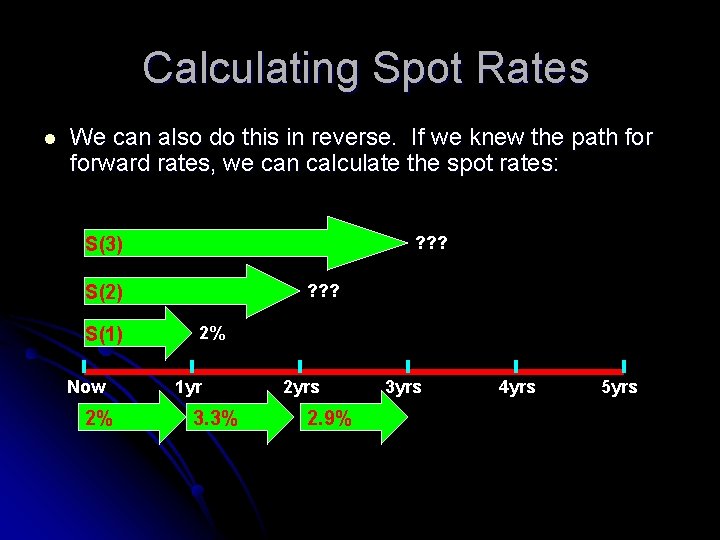
Calculating Spot Rates l We can also do this in reverse. If we knew the path forward rates, we can calculate the spot rates: ? ? ? S(3) ? ? ? S(2) S(1) Now 2% 2% 1 yr 3. 3% 2 yrs 2. 9% 3 yrs 4 yrs 5 yrs

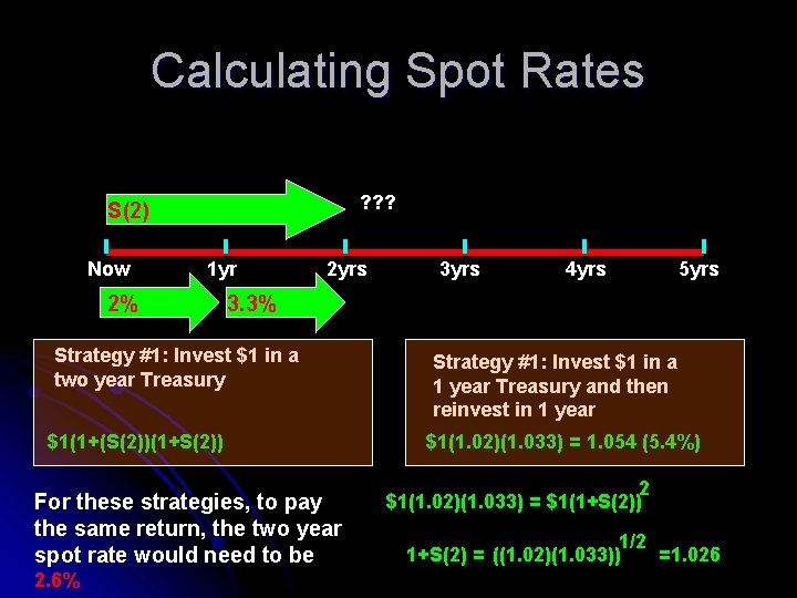
Calculating Spot Rates ? ? ? S(2) Now 1 yr 2% 2 yrs 4 yrs 5 yrs 3. 3% Strategy #1: Invest $1 in a two year Treasury $1(1+(S(2))(1+S(2)) For these strategies, to pay the same return, the two year spot rate would need to be 2. 6% 3 yrs Strategy #1: Invest $1 in a 1 year Treasury and then reinvest in 1 year $1(1. 02)(1. 033) = 1. 054 (5. 4%) 2 $1(1. 02)(1. 033) = $1(1+S(2)) 1/2 1+S(2) = ((1. 02)(1. 033)) =1. 026

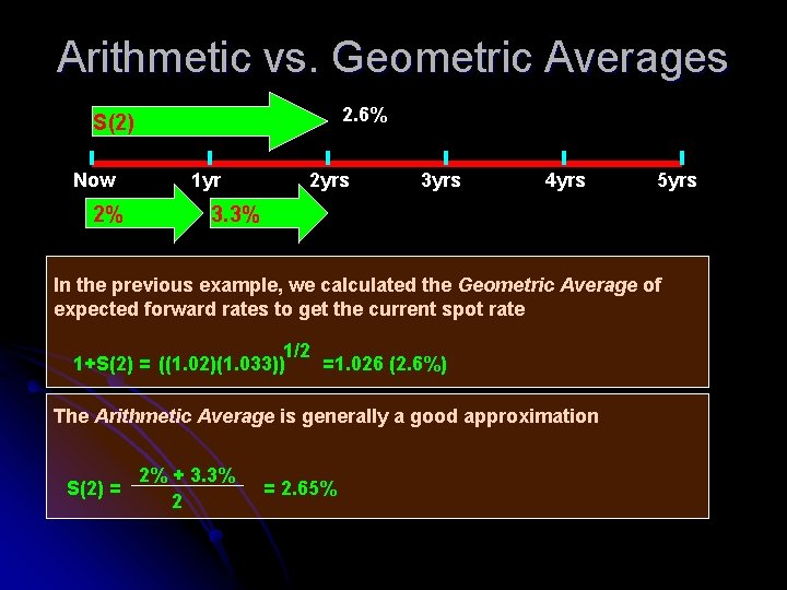
Arithmetic vs. Geometric Averages 2. 6% S(2) Now 2% 1 yr 2 yrs 3 yrs 4 yrs 5 yrs 3. 3% In the previous example, we calculated the Geometric Average of expected forward rates to get the current spot rate 1/2 1+S(2) = ((1. 02)(1. 033)) =1. 026 (2. 6%) The Arithmetic Average is generally a good approximation S(2) = 2% + 3. 3% 2 = 2. 65%

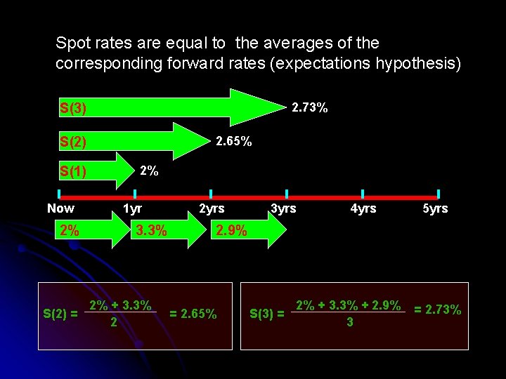
Spot rates are equal to the averages of the corresponding forward rates (expectations hypothesis) 2. 73% S(3) 2. 65% S(2) S(1) Now 2% S(2) = 2% 1 yr 3. 3% 2% + 3. 3% 2 2 yrs 3 yrs 4 yrs 5 yrs 2. 9% = 2. 65% S(3) = 2% + 3. 3% + 2. 9% 3 = 2. 73%

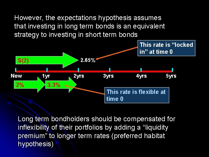
However, the expectations hypothesis assumes that investing in long term bonds is an equivalent strategy to investing in short term bonds This rate is “locked in” at time 0 2. 65% S(2) Now 2% 1 yr 2 yrs 3 yrs 4 yrs 5 yrs 3. 3% This rate is flexible at time 0 Long term bondholders should be compensated for inflexibility of their portfolios by adding a “liquidity premium” to longer term rates (preferred habitat hypothesis)

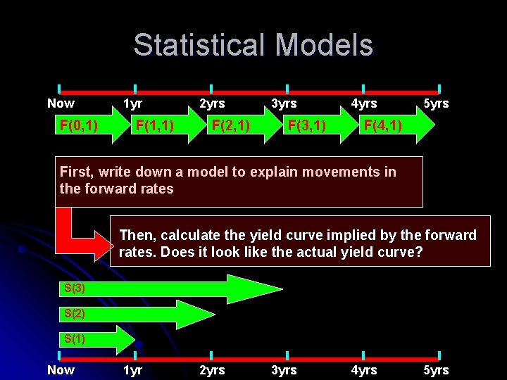
Statistical Models Now F(0, 1) 1 yr F(1, 1) 2 yrs F(2, 1) 3 yrs F(3, 1) 4 yrs 5 yrs 3. 3% F(4, 1) First, write down a model to explain movements in the forward rates Then, calculate the yield curve implied by the forward rates. Does it look like the actual yield curve? S(3) S(2) S(1) Now 1 yr 2 yrs 3 yrs 4 yrs 5 yrs

Lattice Methods (Discrete) l Lattice models assume that the interest rate makes discrete jumps between time periods (usually calibrated monthly) l Binomial: Two Possibilities each Period l Trinomial: Three Possibilities each Period

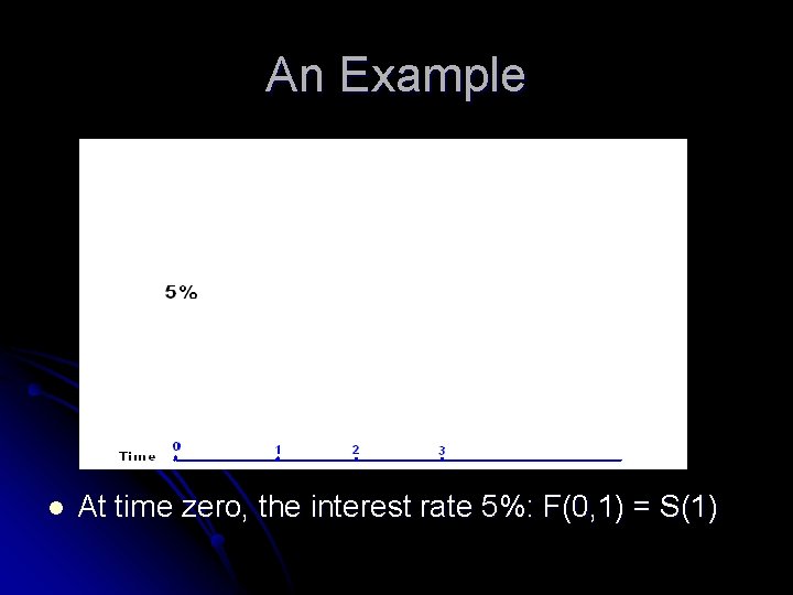
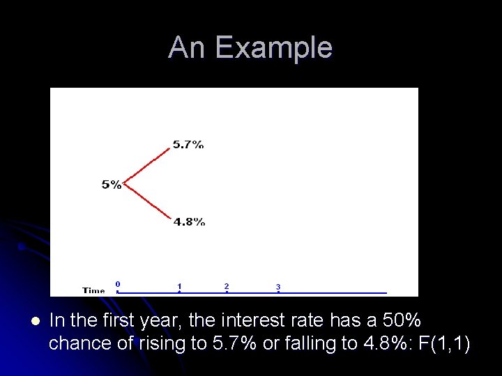
An Example l At time zero, the interest rate 5%: F(0, 1) = S(1)

An Example l In the first year, the interest rate has a 50% chance of rising to 5. 7% or falling to 4. 8%: F(1, 1)

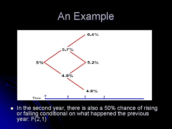
An Example l In the second year, there is also a 50% chance of rising or falling conditional on what happened the previous year: F(2, 1)

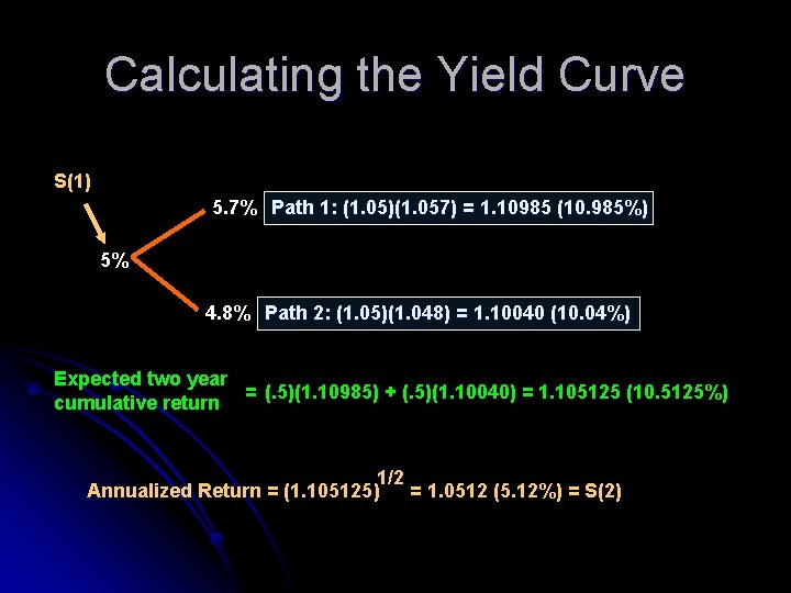
Calculating the Yield Curve S(1) 5. 7% Path 1: (1. 05)(1. 057) = 1. 10985 (10. 985%) 5% 4. 8% Path 2: (1. 05)(1. 048) = 1. 10040 (10. 04%) Expected two year = (. 5)(1. 10985) + (. 5)(1. 10040) = 1. 105125 (10. 5125%) cumulative return 1/2 Annualized Return = (1. 105125) = 1. 0512 (5. 12%) = S(2)

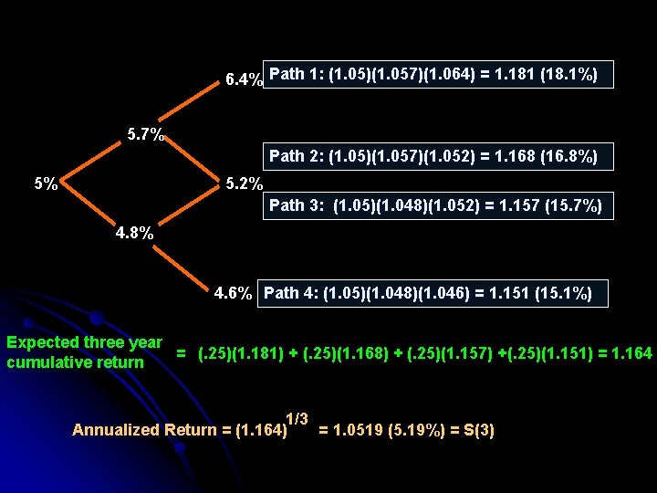
6. 4% Path 1: (1. 05)(1. 057)(1. 064) = 1. 181 (18. 1%) 5. 7% Path 2: (1. 05)(1. 057)(1. 052) = 1. 168 (16. 8%) 5% 5. 2% Path 3: (1. 05)(1. 048)(1. 052) = 1. 157 (15. 7%) 4. 8% 4. 6% Path 4: (1. 05)(1. 048)(1. 046) = 1. 151 (15. 1%) Expected three year = (. 25)(1. 181) + (. 25)(1. 168) + (. 25)(1. 157) +(. 25)(1. 151) = 1. 164 cumulative return 1/3 Annualized Return = (1. 164) = 1. 0519 (5. 19%) = S(3)

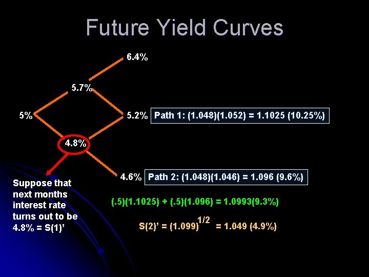
Future Yield Curves 6. 4% 5. 7% 5% 5. 2% Path 1: (1. 048)(1. 052) = 1. 1025 (10. 25%) 4. 8% Suppose that next months interest rate turns out to be 4. 8% = S(1)’ 4. 6% Path 2: (1. 048)(1. 046) = 1. 096 (9. 6%) (. 5)(1. 1025) + (. 5)(1. 096) = 1. 0993(9. 3%) 1/2 S(2)’ = (1. 099) = 1. 049 (4. 9%)

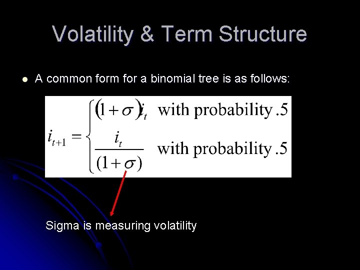
Volatility & Term Structure l A common form for a binomial tree is as follows: Sigma is measuring volatility

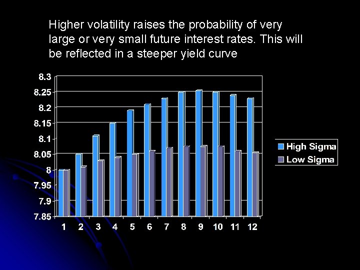
Higher volatility raises the probability of very large or very small future interest rates. This will be reflected in a steeper yield curve

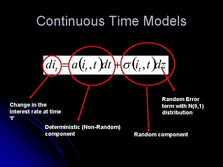
Continuous Time Models Change in the interest rate at time ‘t’ Deterministic (Non-Random) component Random Error term with N(0, 1) distribution Random component

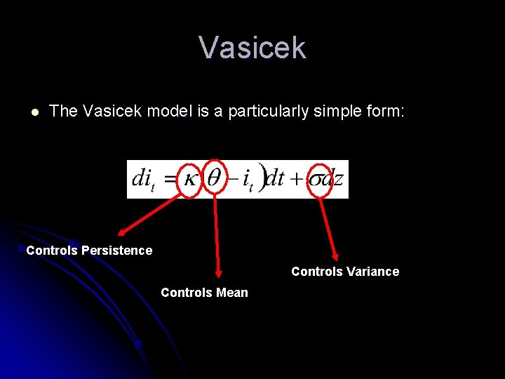
Vasicek l The Vasicek model is a particularly simple form: Controls Persistence Controls Variance Controls Mean

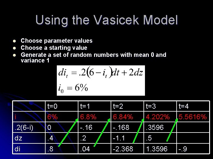
Using the Vasicek Model l Choose parameter values Choose a starting value Generate a set of random numbers with mean 0 and variance 1 i. 2(6 -i) t=0 6% 0 t=1 6. 8% -. 16 t=2 6. 84% -. 168 t=3 4. 202%. 3596 dz di . 4. 8 . 2. 04 -1. 1 -2. 368 . 5 1. 3596 t=4 5. 5616% -. 9

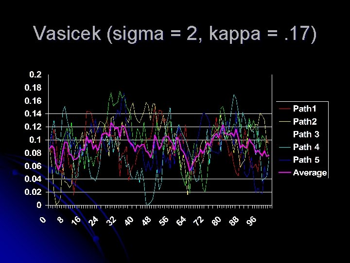
Vasicek (sigma = 2, kappa =. 17)

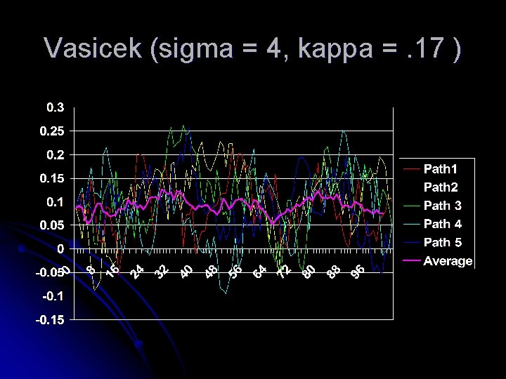
Vasicek (sigma = 4, kappa =. 17 )

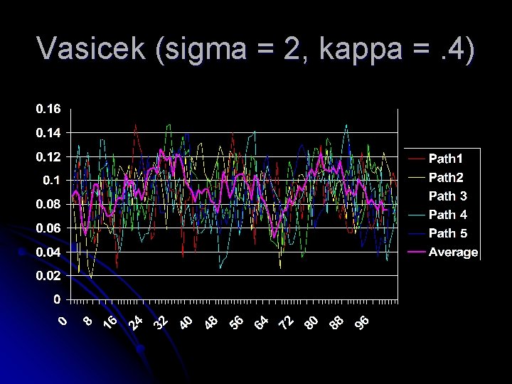
Vasicek (sigma = 2, kappa =. 4)

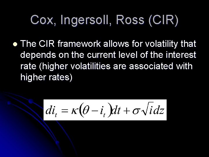
Cox, Ingersoll, Ross (CIR) l The CIR framework allows for volatility that depends on the current level of the interest rate (higher volatilities are associated with higher rates)

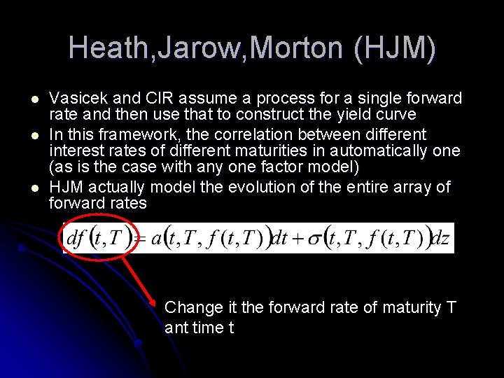
Heath, Jarow, Morton (HJM) l l l Vasicek and CIR assume a process for a single forward rate and then use that to construct the yield curve In this framework, the correlation between different interest rates of different maturities in automatically one (as is the case with any one factor model) HJM actually model the evolution of the entire array of forward rates Change it the forward rate of maturity T ant time t

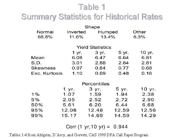
Table 1 Summary Statistics for Historical Rates Tables 1 -4 from Ahlgrim, D’Arcy, and Gorvett, CAS 1999 DFA Call Paper Program

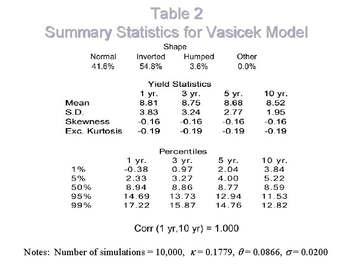
Table 2 Summary Statistics for Vasicek Model Notes: Number of simulations = 10, 000, k = 0. 1779, q = 0. 0866, s = 0. 0200

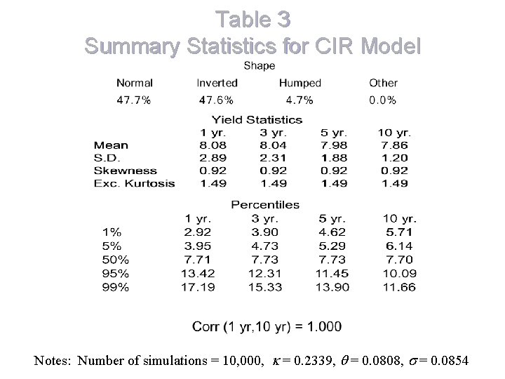
Table 3 Summary Statistics for CIR Model Notes: Number of simulations = 10, 000, k = 0. 2339, q = 0. 0808, s = 0. 0854

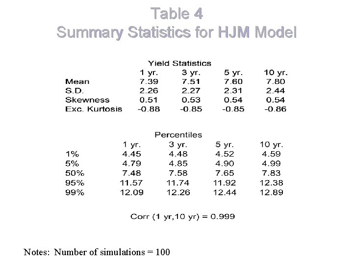
Table 4 Summary Statistics for HJM Model Notes: Number of simulations = 100