Predicting House Prices with Spatial Dependence A Comparison

Predicting House Prices with Spatial Dependence: A Comparison of Alternative Methods Steven C. Bourassa University of Louisville (USA) and Bordeaux Management School (France) Eva Cantoni University of Geneva (Switzerland) Martin Hoesli University of Geneva (Switzerland), University of Aberdeen (U. K. ), and Bordeaux Management School (France) European Real Estate Society Annual Conference Stockholm, Sweden 24 -27 June 2009

Outline of Paper • • • Purpose of Study Research Design Data Empirical Results Conclusions 2

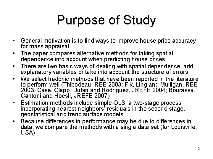
Purpose of Study • General motivation is to find ways to improve house price accuracy for mass appraisal • The paper compares alternative methods for taking spatial dependence into account when predicting house prices • There are two basic ways of dealing with spatial dependence: add explanatory variables or take into account the structure of errors • We select hedonic methods that have been reported in the literature to perform well (Thibodeau, REE 2003; Fik, Ling and Mulligan, REE 2003; Case, Clapp, Dubin and Rodriguez, JREFE 2004; Bourassa, Cantoni and Hoesli, JREFE 2007) • Estimation methods include simple OLS, a two-stage process incorporating nearest neighbors’ residuals in the second stage, geostatistical and trend surface models • Because differences in performance may be due to differences in data, we compare the methods with a single data set (for Louisville, USA) 3

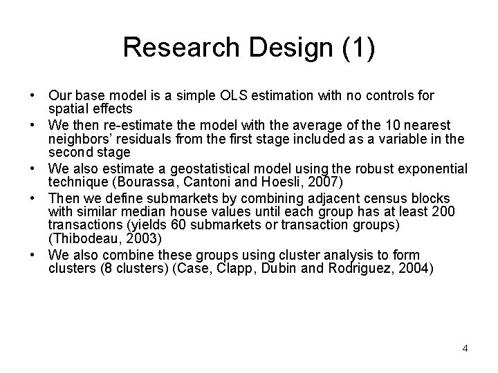
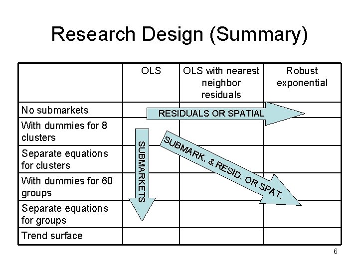
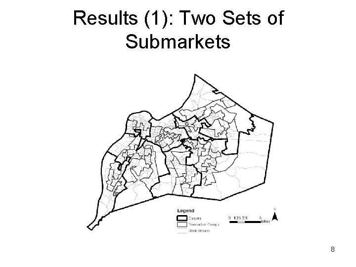
Research Design (1) • Our base model is a simple OLS estimation with no controls for spatial effects • We then re-estimate the model with the average of the 10 nearest neighbors’ residuals from the first stage included as a variable in the second stage • We also estimate a geostatistical model using the robust exponential technique (Bourassa, Cantoni and Hoesli, 2007) • Then we define submarkets by combining adjacent census blocks with similar median house values until each group has at least 200 transactions (yields 60 submarkets or transaction groups) (Thibodeau, 2003) • We also combine these groups using cluster analysis to form clusters (8 clusters) (Case, Clapp, Dubin and Rodriguez, 2004) 4

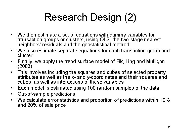
Research Design (2) • We then estimate a set of equations with dummy variables for transaction groups or clusters, using OLS, the two-stage nearest neighbors’ residuals and the geostatistical method • We also estimate separate equations for each transaction group and cluster • Finally, we apply the trend surface model of Fik, Ling and Mulligan (2003) • This involves including the squares and cubes of selected property attributes as well as the x- and y-coordinates and their squares and cubes, as well as interactions of these variables • Each model is estimated using 100 random samples of the data • Out-of-sample predictions • We calculate error statistics and proportion of predictions within 10% and 20% of sale price 5

Research Design (Summary) OLS No submarkets Separate equations for clusters With dummies for 60 groups Separate equations for groups Robust exponential RESIDUALS OR SPATIAL SUBMARKETS With dummies for 8 clusters OLS with nearest neighbor residuals SU BM AR K. &R ES ID. OR SP AT. Trend surface 6

Data • House price data from Property Valuation Administrator of Jefferson County (Louisville), Kentucky, USA • Records include sale prices and property attributes • Data for all single-family houses sold in 1999 (n = 12, 982) 7

Results (1): Two Sets of Submarkets 8

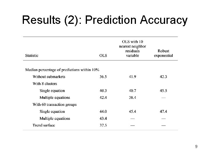
Results (2): Prediction Accuracy 9

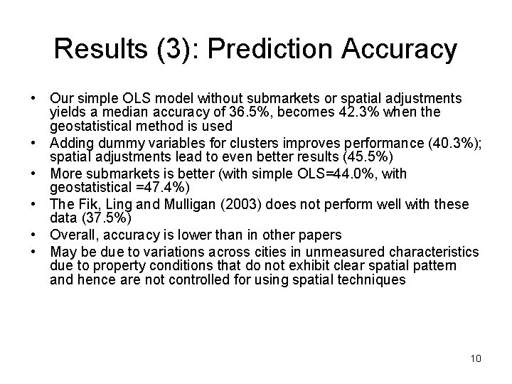
Results (3): Prediction Accuracy • Our simple OLS model without submarkets or spatial adjustments yields a median accuracy of 36. 5%, becomes 42. 3% when the geostatistical method is used • Adding dummy variables for clusters improves performance (40. 3%); spatial adjustments lead to even better results (45. 5%) • More submarkets is better (with simple OLS=44. 0%, with geostatistical =47. 4%) • The Fik, Ling and Mulligan (2003) does not perform well with these data (37. 5%) • Overall, accuracy is lower than in other papers • May be due to variations across cities in unmeasured characteristics due to property conditions that do not exhibit clear spatial pattern and hence are not controlled for using spatial techniques 10

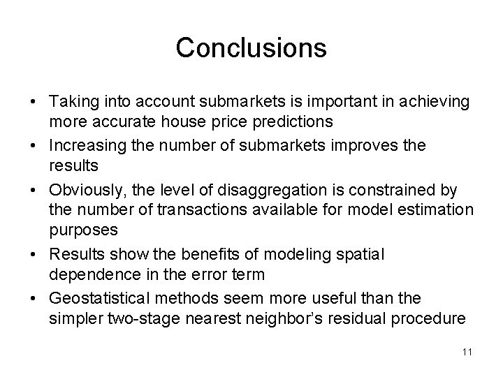
Conclusions • Taking into account submarkets is important in achieving more accurate house price predictions • Increasing the number of submarkets improves the results • Obviously, the level of disaggregation is constrained by the number of transactions available for model estimation purposes • Results show the benefits of modeling spatial dependence in the error term • Geostatistical methods seem more useful than the simpler two-stage nearest neighbor’s residual procedure 11