Predicting Conditional Branches With FusionBased Hybrid Predictors Gabriel

Predicting Conditional Branches With Fusion-Based Hybrid Predictors Gabriel H. Loh Yale University Dept. of Computer Science Dana S. Henry Yale University Depts. of Elec. Eng. & Comp. Sci. This research was funded by NSF Grant MIP-9702281

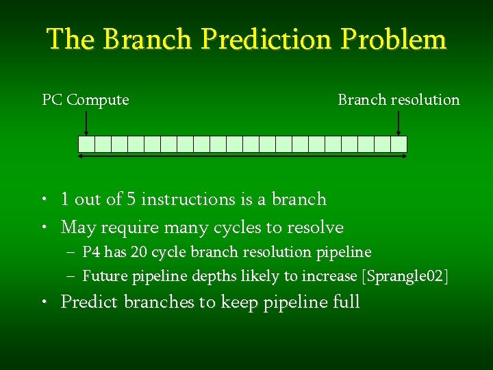
The Branch Prediction Problem PC Compute • • Branch resolution 1 out of 5 instructions is a branch May require many cycles to resolve – P 4 has 20 cycle branch resolution pipeline – Future pipeline depths likely to increase [Sprangle 02] • Predict branches to keep pipeline full

Bigger Predictors = More Accurate (but bigger predictors = slower) • Larger predictors tend to yield more accurate predictions • Faster cycle times force smaller branch predictors • Overriding predictor couples small, fast predictor with a large, multi-cycle predictor [Jiménez 2000] – performs close to ideal large-fast predictor

Hybrid Predictors • Wide variety of branch prediction algorithms available • Hybrid combines more than one “stand-alone” or component predictor [Mc. Farling 93]: Meta. Predictor P 1 P 2 Final Prediction

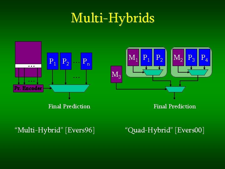
Multi-Hybrids … … M 1 P 2 P 1 P 2 … Pn … M 2 P 3 P 4 M 3 Pr. Encoder Final Prediction “Multi-Hybrid” [Evers 96] Final Prediction “Quad-Hybrid” [Evers 00]

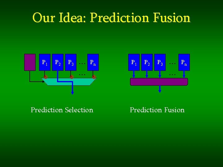
Our Idea: Prediction Fusion P 1 X P 2 P 3 X … Pn … X Prediction Selection P 1 P 2 P 3 … Pn … Prediction Fusion

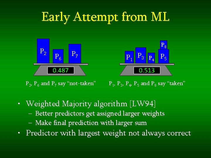
Early Attempt from ML P 2 P 6 P 7 P 8 P 1 P 3 P 4 P 5 0. 487 0. 513 P 2, P 6 and P 7 say “not-taken” P 1, P 3, P 4, P 5 and P 8 say “taken” • Weighted Majority algorithm [LW 94] – – Better predictors get assigned larger weights Make final prediction with larger sum • Predictor with largest weight not always correct

Outline • • COLT Predictor Choosing parameters and components Performance Prediction distributions, component choice

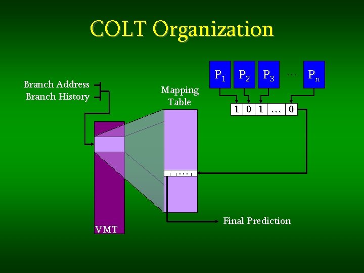
COLT Organization Branch Address Branch History Mapping Table P 1 P 2 P 3 … Pn 1 0 1 … 0 … VMT Final Prediction

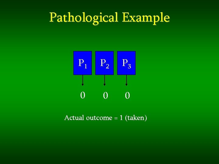
Pathological Example P 1 P 2 P 3 0 0 0 Actual outcome = 1 (taken)

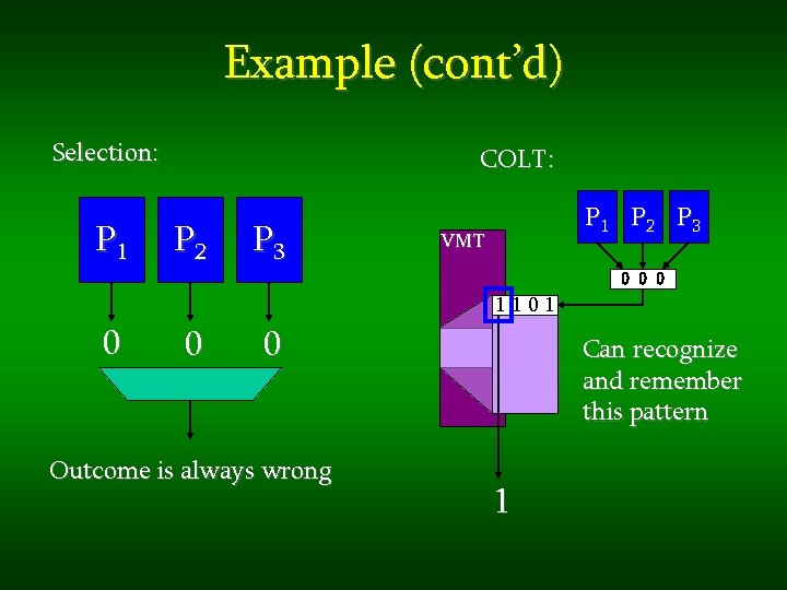
Example (cont’d) Selection: P 1 COLT: P 2 P 3 P 1 P 2 P 3 VMT 0 0 0 1101 0 0 0 Outcome is always wrong Can recognize and remember this pattern 1

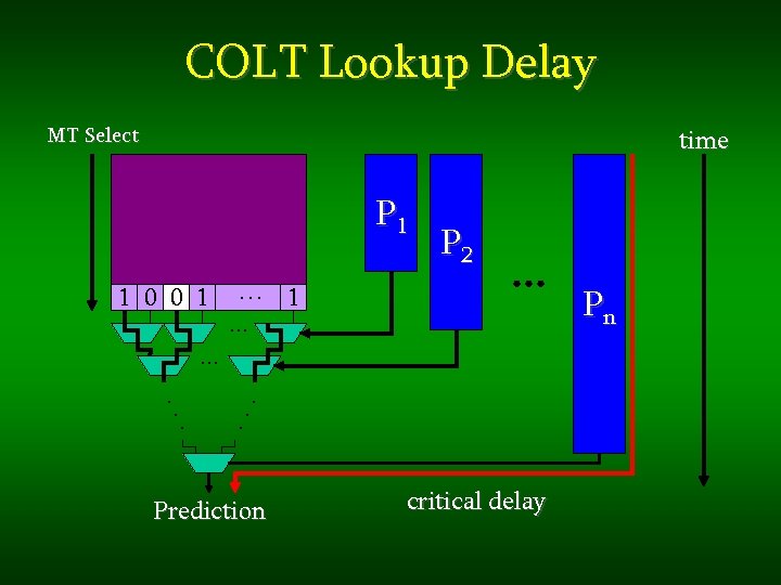
COLT Lookup Delay MT Select time P 1 1 0 0 1. . . … 1. . . P 2 … . . . Prediction critical delay Pn

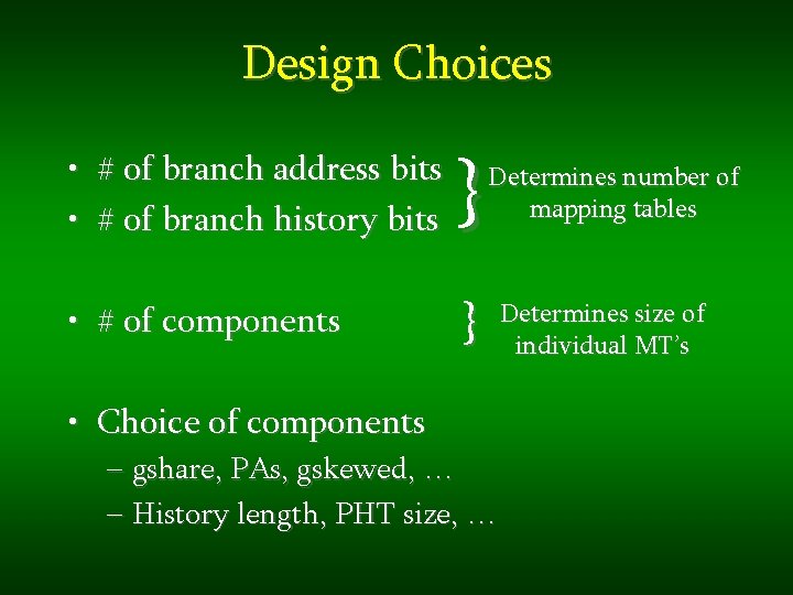
Design Choices • # of branch address bits • # of branch history bits } • # of components } Determines number of mapping tables • Choice of components – gshare, PAs, gskewed, … – History length, PHT size, … Determines size of individual MT’s

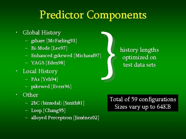
Predictor Components • Global History – – • Local History – PAs [Yeh 94] – pskewed [Evers 96] • Other – – – } gshare [Mc. Farling 93] Bi-Mode [Lee 97] Enhanced gskewed [Michaud 97] YAGS [Eden 98] 2 b. C (bimodal) [Smith 81] Loop [Chang 95] alloyed Perceptron [Jiménez 02] history lengths optimized on test data sets Total of 59 configurations Sizes vary up to 64 KB

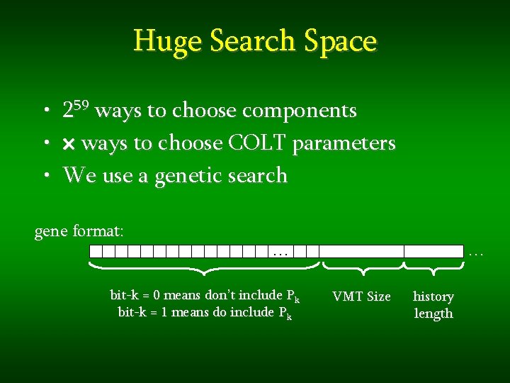
Huge Search Space • • • 259 ways to choose components ways to choose COLT parameters We use a genetic search gene format: … … bit-k = 0 means don’t include Pk bit-k = 1 means do include Pk VMT Size history length

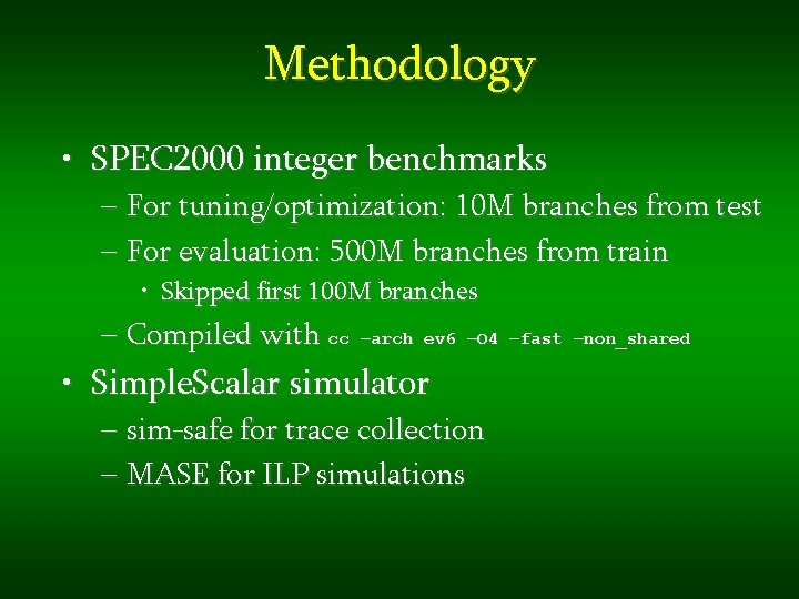
Methodology • SPEC 2000 integer benchmarks – For tuning/optimization: 10 M branches from test – For evaluation: 500 M branches from train • Skipped first 100 M branches – Compiled with cc –arch ev 6 –O 4 –fast –non_shared • Simple. Scalar simulator – sim-safe for trace collection – MASE for ILP simulations

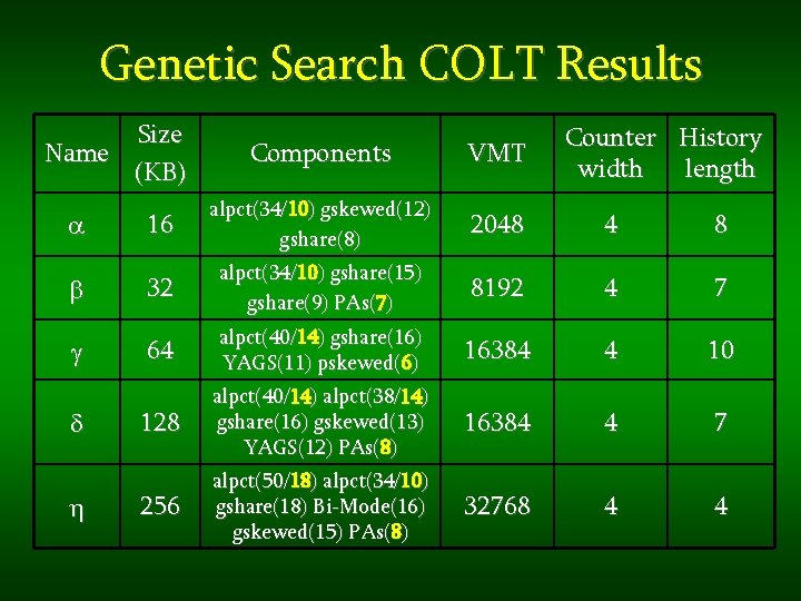
Genetic Search COLT Results Size Name (KB) Counter History width length Components VMT 16 alpct(34/10) gskewed(12) gshare(8) 2048 4 8 b 32 alpct(34/10) gshare(15) gshare(9) PAs(7) 8192 4 7 g 64 alpct(40/14) gshare(16) YAGS(11) pskewed(6) 16384 4 10 128 alpct(40/14) alpct(38/14) gshare(16) gskewed(13) YAGS(12) PAs(8) 16384 4 7 256 alpct(50/18) alpct(34/10) gshare(18) Bi-Mode(16) gskewed(15) PAs(8) 32768 4 4 a d h

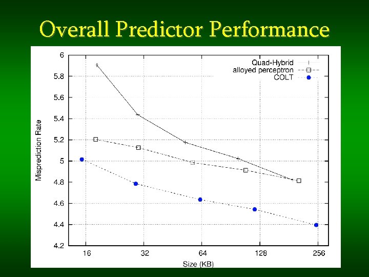
Overall Predictor Performance

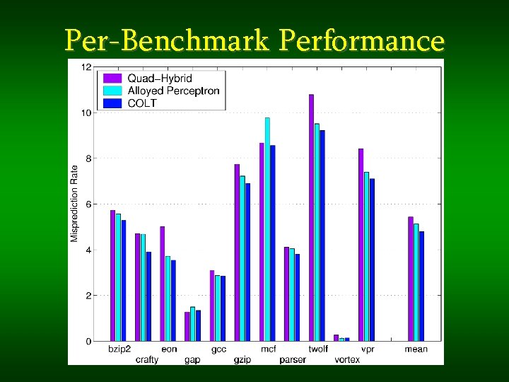
Per-Benchmark Performance

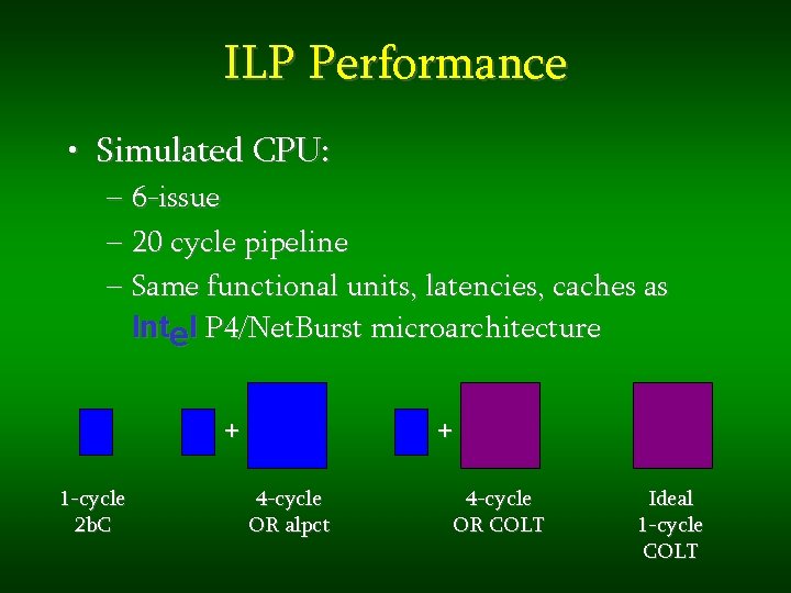
ILP Performance • Simulated CPU: – 6 -issue – 20 cycle pipeline – Same functional units, latencies, caches as Intel P 4/Net. Burst microarchitecture + 1 -cycle 2 b. C + 4 -cycle OR alpct 4 -cycle OR COLT Ideal 1 -cycle COLT

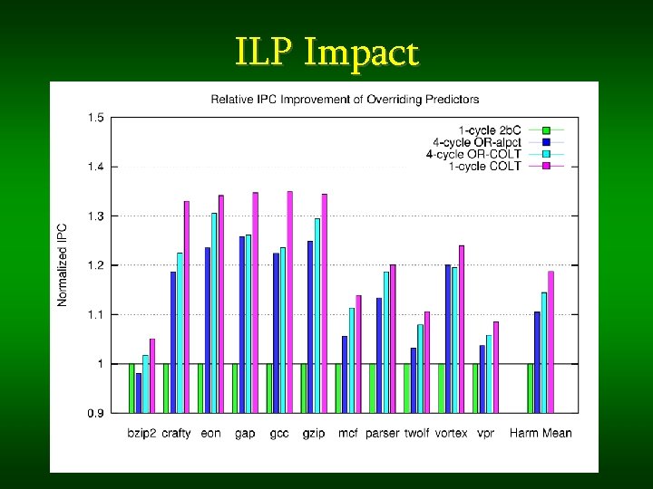
ILP Impact

COLT Parameter Sensitivity • • • Mapping table counter widths Number of mapping tables Number of history bits for VMT index

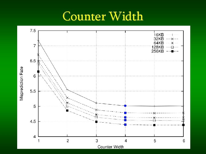
Counter Width

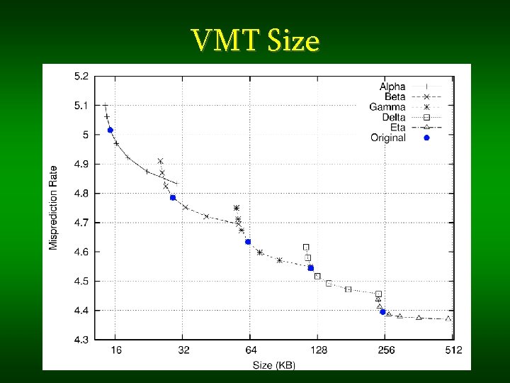
VMT Size

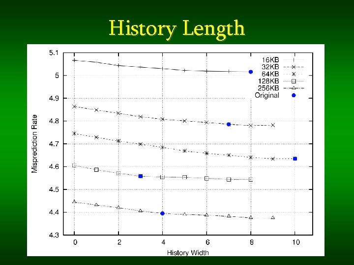
History Length

Explaining Choice of Components • Parameter sensitivity results shows GA performed well for the COLT parameters • Why did it choose the component predictors that it did?

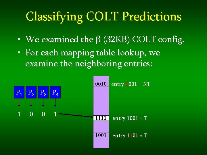
Classifying COLT Predictions • We examined the b (32 KB) COLT config. • For each mapping table lookup, we examine the neighboring entries: P 1 P 2 P 3 P 4 1 0 0 1 0010 entry 0001 = NT 1111 entry 1001 = T 1001 entry 1101 = T

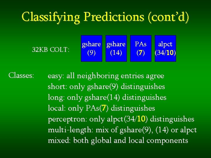
Classifying Predictions (cont’d) 32 KB COLT: Classes: gshare (9) (14) PAs ( 7) alpct (34/10) easy: all neighboring entries agree short: only gshare(9) distinguishes long: only gshare(14) distinguishes local: only PAs(7) distinguishes perceptron: only alpct(34/10) distinguishes multi-length: mix of gshare(9), (14) or alpct mixed: both global and local components

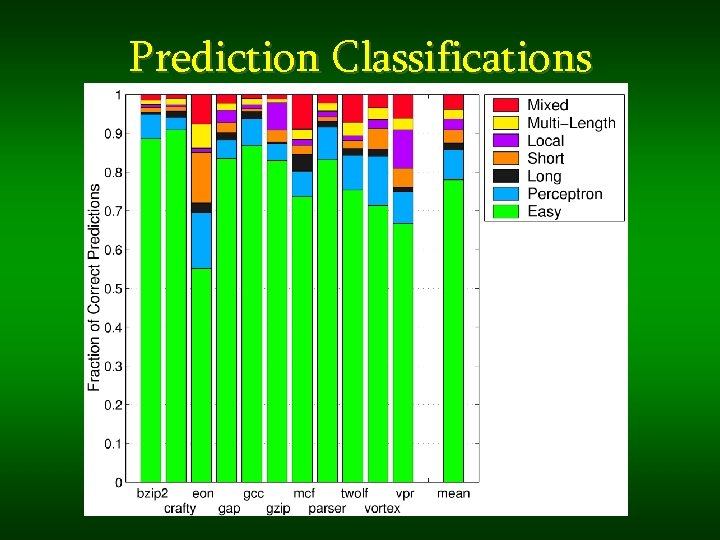
Prediction Classifications

Related Work/Issues • • Alloyed history [Skadron 00] Variable path history length [Stark 98] Dynamic history length fitting [Juan 98] Interference reduction [lots…] ü COLT handles all of these cases* ODoesn’t support partial update policies

Open Research • • • Better individual components Augment with SBI [Manne 99], agree [Sprangle 97] Better fusion algorithms Hybrid fusion/selection algorithms Other domains (branch confidence prediction, value prediction, memory dependence prediction, instruction criticality prediction, …)

Summary • Fusion is more powerful than selection – Combines multiple sources of information • Branch behavior is very varied – Need long, short, global and local histories, multiple simultaneous lengths and types of history • COLT is one possible fusion-based predictor – Combines multiple types of information – Current “best” purely dynamic predictor*

Questions?