Predictability of Japan East Sea JES System to

Predictability of Japan / East Sea (JES) System to Uncertain Initial / Lateral Boundary Conditions and Surface Winds LCDR. Chin-Lung Fang

Outline • • • Introduction Experimental design Statistical analysis methods Results Conclusions

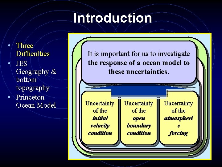
Introduction • Three Difficulties • JES Geography & bottom topography • Princeton Ocean Model Numerical ocean modeling It is important for us to investigate the response. Initial of a-ocean and model to Boundary -value problems these uncertainties. Three major difficulties Uncertainty of the initial velocity condition Uncertainty of the open boundary condition Uncertainty of the atmospheri c forcing

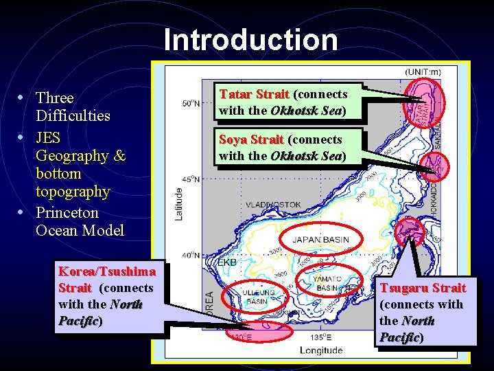
Introduction • Three Difficulties • JES Geography & bottom topography • Princeton Ocean Model Korea/Tsushima Strait (connects with the North Pacific) Pacific Tatar Strait (connects with the Okhotsk Sea) Sea Soya Strait (connects with the Okhotsk Sea) Sea Tsugaru Strait (connects with the North Pacific) Pacific

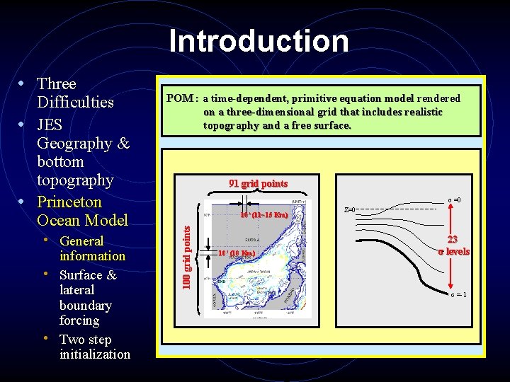
Introduction Difficulties • JES Geography & bottom topography • Princeton Ocean Model • General information • Surface & lateral boundary forcing • Two step initialization POM : a time-dependent, primitive equation model rendered on a three-dimensional grid that includes realistic topography and a free surface. 91 grid points σ =0 10’ (11~15 Km) 100 grid points • Three 10’ (18 Km) Z=0 23 σ levels σ =-1

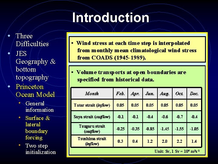
Introduction • Three Difficulties • JES Geography & bottom topography • Princeton Ocean Model • General information • Surface & lateral boundary forcing • Two step initialization • Wind stress at each time step is interpolated from monthly mean climatological wind stress from COADS (1945 -1989). • Volume transports at open boundaries are specified from historical data. Month Feb. Apr. Jun. Aug. Oct. Dec. Tatar strait (inflow) 0. 05 Soya strait (outflow) -0. 1 -0. 4 -0. 6 -0. 7 -0. 4 Tsugaru strait (outflow) -0. 25 -0. 35 -0. 85 -1. 45 -1. 55 -1. 05 Tsushima strait (inflow) 0. 3 0. 4 1. 2 2. 0 2. 2 1. 4 Unit: Sv, 1 Sv = 106 m 3 s-1

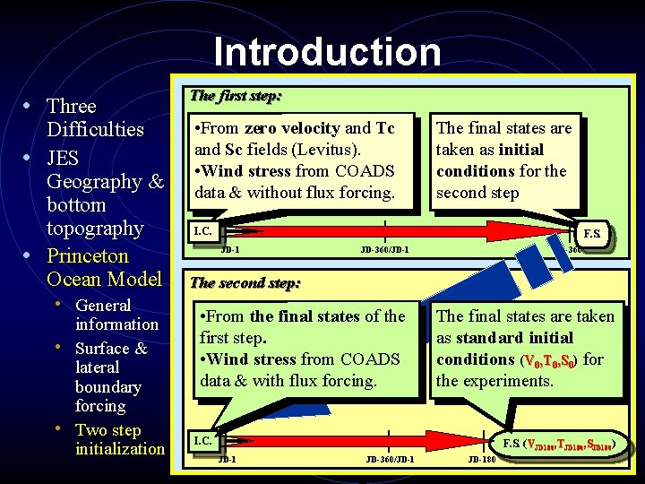
Introduction • Three Difficulties • JES Geography & bottom topography • Princeton Ocean Model • General information • Surface & lateral boundary forcing • Two step initialization The first step: • From zero velocity and Tc and Sc fields (Levitus). • Wind stress from COADS data & without flux forcing. The final states are taken as initial conditions for the second step I. C. F. S. JD-1 JD-360/JD-1 JD-360 The second step: • From the final states of the first step. • Wind stress from COADS data & with flux forcing. The final states are taken as standard initial conditions (V 0, T 0, S 0) for the experiments. I. C. F. S. (V VJD 180, TJD 180, SJD 180) JD-1 JD-360/JD-180

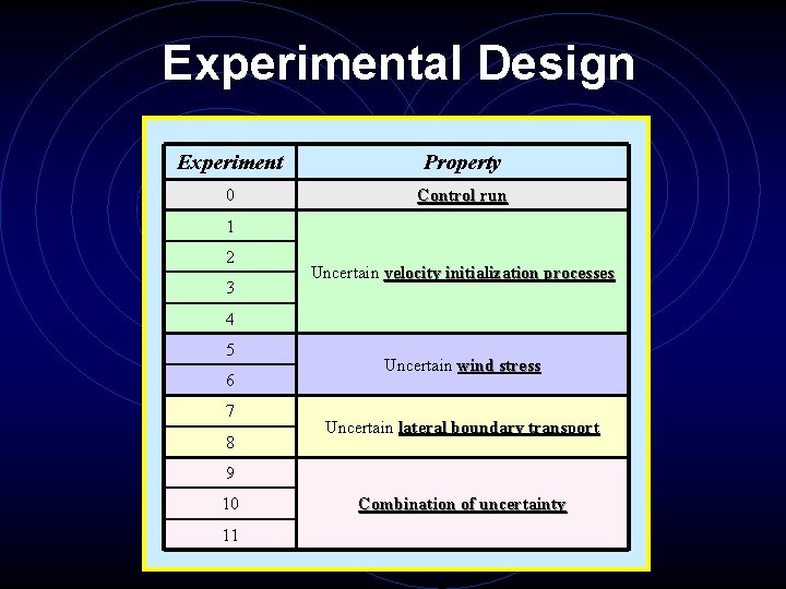
Experimental Design Experiment Property 0 Control run 1 2 3 Uncertain velocity initialization processes 4 5 6 7 8 Uncertain wind stress Uncertain lateral boundary transport 9 10 11 Combination of uncertainty

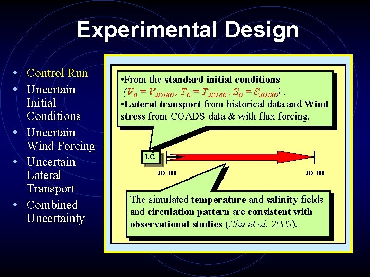
Experimental Design • Control Run • Uncertain • • • Initial Conditions Uncertain Wind Forcing Uncertain Lateral Transport Combined Uncertainty • From the standard initial conditions (V 0 = VJD 180 , T 0 = TJD 180 , S 0 = SJD 180). • Lateral transport from historical data and Wind stress from COADS data & with flux forcing. I. C. JD-180 JD-360 The simulated temperature and salinity fields and circulation pattern are consistent with observational studies (Chu et al. 2003).

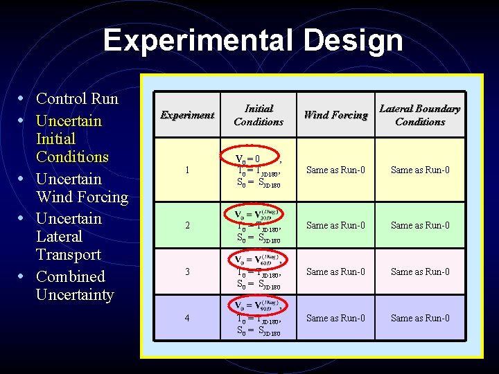
Experimental Design • Control Run • Uncertain • • • Initial Conditions Uncertain Wind Forcing Uncertain Lateral Transport Combined Uncertainty Experiment Initial Conditions Wind Forcing Lateral Boundary Conditions 1 V 0 = 0 , T 0 = TJD 180, S 0 = SJD 180 Same as Run-0 2 T 0 = TJD 180, S 0 = SJD 180 Same as Run-0 3 T 0 = TJD 180, S 0 = SJD 180 Same as Run-0 4 T 0 = TJD 180, S 0 = SJD 180 Same as Run-0

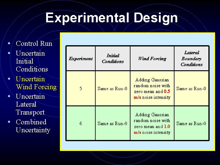
Experimental Design • Control Run • Uncertain • • • Initial Conditions Uncertain Wind Forcing Uncertain Lateral Transport Combined Uncertainty Experiment 5 6 Initial Conditions Wind Forcing Lateral Boundary Conditions Same as Run-0 Adding Gaussian random noise with zero mean and 0. 5 m/s noise intensity Same as Run-0 Adding Gaussian random noise with zero mean and 1. 0 m/s noise intensity Same as Run-0

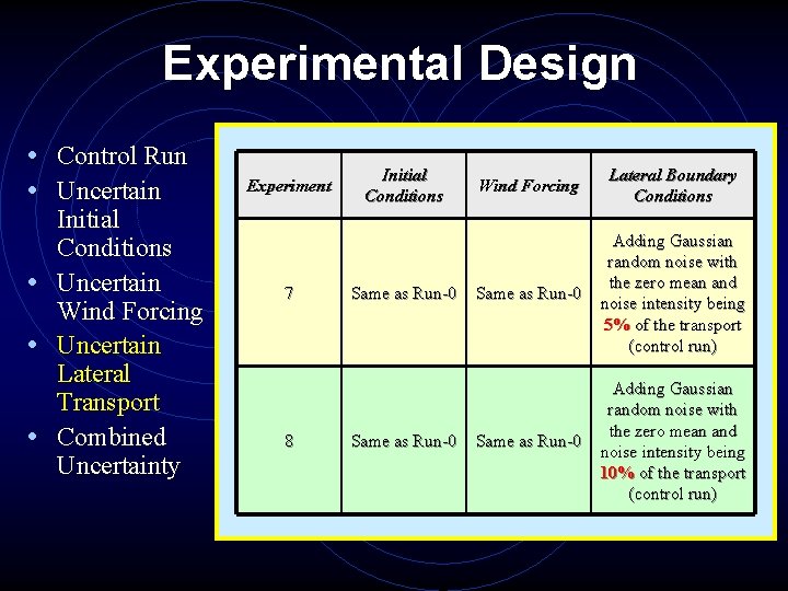
Experimental Design • Control Run • Uncertain • • • Initial Conditions Uncertain Wind Forcing Uncertain Lateral Transport Combined Uncertainty Experiment 7 8 Initial Conditions Same as Run-0 Wind Forcing Lateral Boundary Conditions Same as Run-0 Adding Gaussian random noise with the zero mean and noise intensity being 5% of the transport (control run) Same as Run-0 Adding Gaussian random noise with the zero mean and noise intensity being 10% of the transport (control run)

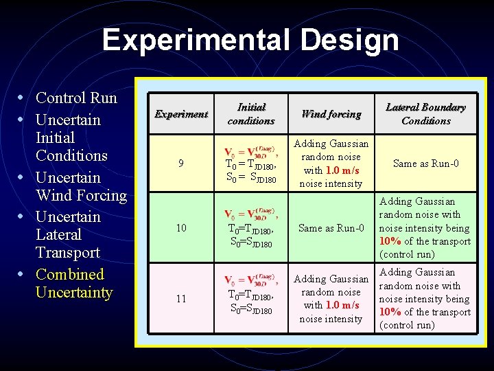
Experimental Design • Control Run • Uncertain • • • Initial Conditions Uncertain Wind Forcing Uncertain Lateral Transport Combined Uncertainty Experiment 9 10 11 Initial conditions T 0 = TJD 180, S 0 = SJD 180 T 0=TJD 180, S 0=SJD 180 Wind forcing Lateral Boundary Conditions Adding Gaussian random noise with 1. 0 m/s noise intensity Same as Run-0 Adding Gaussian random noise with noise intensity being 10% of the transport (control run) Adding Gaussian random noise with random noise intensity being with 1. 0 m/s 10% of the transport noise intensity (control run)

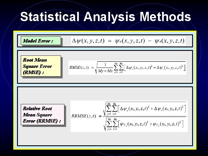
Statistical Analysis Methods Model Error : Root Mean Square Error (RMSE) : Relative Root Mean Square Error (RRMSE) :

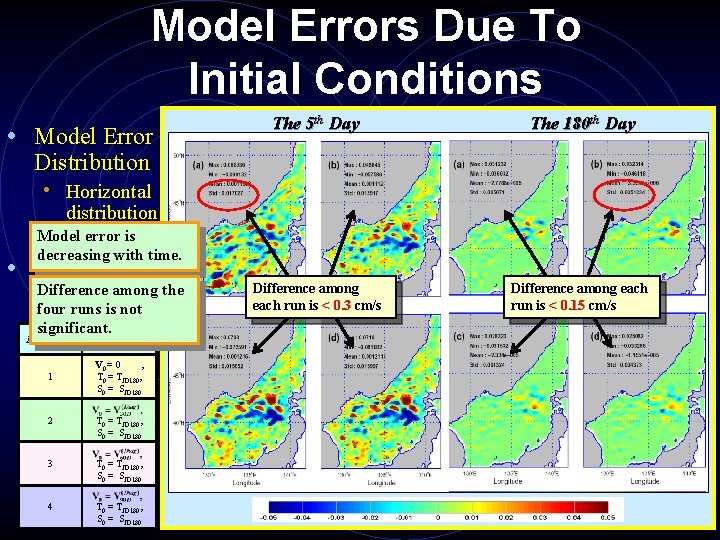
Model Errors Due To Initial Conditions • Model Error The 5 th Day The 180 th Day Difference among each run is < 0. 3 cm/s Difference among each run is < 0. 15 cm/s Distribution • Horizontal distribution Model error is • Histogram decreasing with time. • Relative Difference among the Root Mean four runs is not Square Error significant. Initial Experiment Conditions (RRMSE) 1 V 0 = 0 , T 0 = TJD 180, S 0 = SJD 180 2 T 0 = TJD 180, S 0 = SJD 180 3 T 0 = TJD 180, S 0 = SJD 180 4 T 0 = TJD 180, S 0 = SJD 180

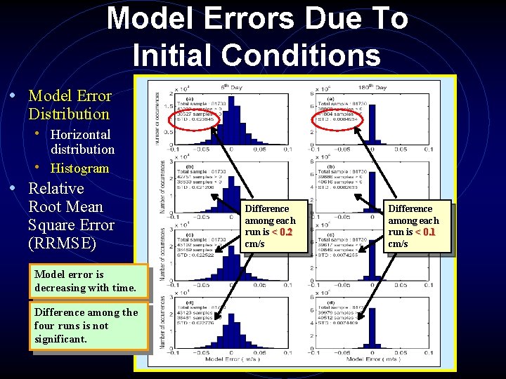
Model Errors Due To Initial Conditions • Model Error Distribution • Horizontal distribution • Histogram • Relative Root Mean Square Error (RRMSE) Model error is decreasing with time. Difference among the four runs is not significant. Difference among each run is < 0. 2 cm/s Difference among each run is < 0. 1 cm/s

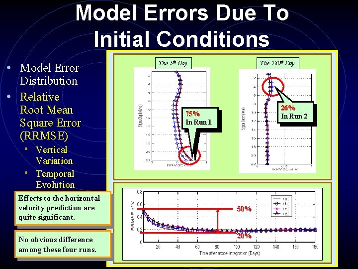
Model Errors Due To Initial Conditions • Model Error Distribution • Relative Root Mean Square Error (RRMSE) The 5 th Day The 180 th Day 26% In Run 2 75% In Run 1 • Vertical Variation • Temporal Evolution Effects to the horizontal velocity prediction are quite significant. No obvious difference among these four runs. 50% 20%

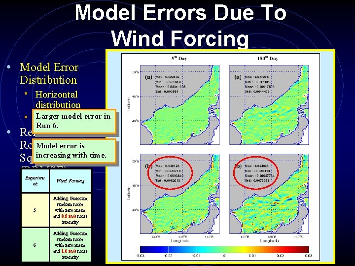
Model Errors Due To Wind Forcing • Model Error Distribution • Horizontal distribution Larger model error in • Histogram Run 6. • Relative Model error is Root Mean increasing with time. Square Error (RRMSE) Experime nt Wind Forcing 5 Adding Gaussian random noise with zero mean and 0. 5 m/s noise intensity 6 Adding Gaussian random noise with zero mean and 1. 0 m/s noise intensity

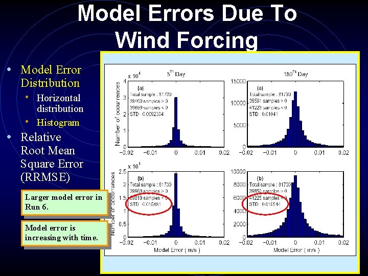
Model Errors Due To Wind Forcing • Model Error Distribution • Horizontal distribution • Histogram • Relative Root Mean Square Error (RRMSE) Larger model error in Run 6. Model error is increasing with time.

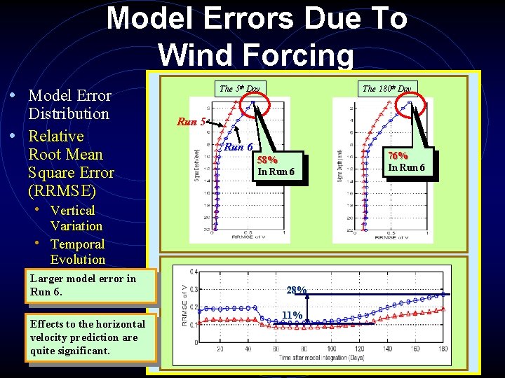
Model Errors Due To Wind Forcing The 5 th Day • Model Error Distribution • Relative Root Mean Square Error (RRMSE) The 180 th Day Run 5 Run 6 58% In Run 6 • Vertical Variation • Temporal Evolution Larger model error in Run 6. Effects to the horizontal velocity prediction are quite significant. 28% 11% 76% In Run 6

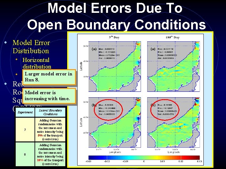
Model Errors Due To Open Boundary Conditions • Model Error Distribution • Horizontal distribution Larger model error in • Histogram Run 8. • Relative error is Root. Model Mean increasing with time. Square Error (RRMSE) Lateral Boundary Experiment Conditions 7 Adding Gaussian random noise with the zero mean and noise intensity being 5% of the transport (control run) 8 Adding Gaussian random noise with the zero mean and noise intensity being 10% of the transport (control run)

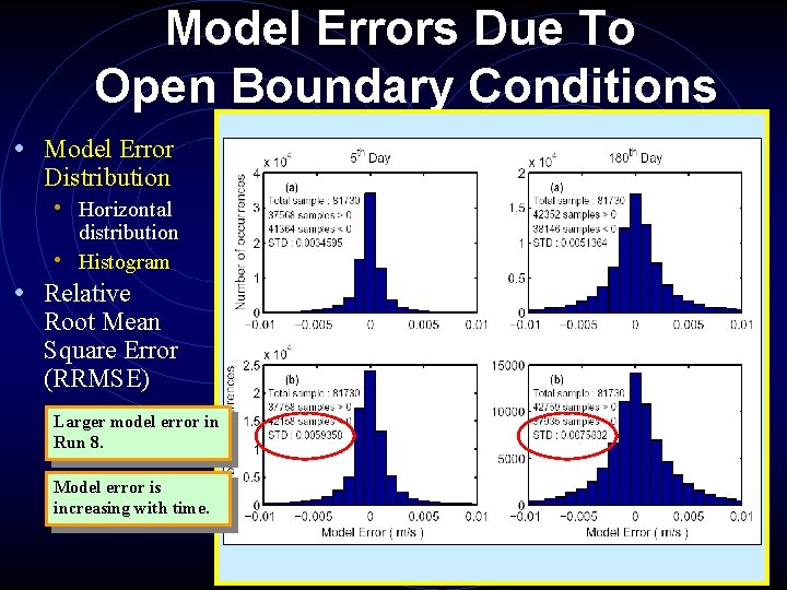
Model Errors Due To Open Boundary Conditions • Model Error Distribution • Horizontal distribution • Histogram • Relative Root Mean Square Error (RRMSE) Larger model error in Run 8. Model error is increasing with time.

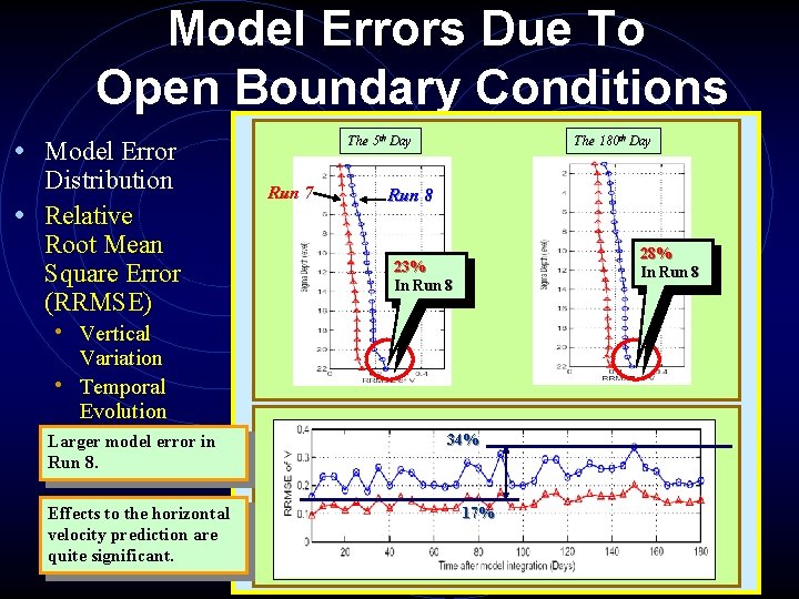
Model Errors Due To Open Boundary Conditions The 5 th Day • Model Error Distribution • Relative Root Mean Square Error (RRMSE) Run 7 The 180 th Day Run 8 28% In Run 8 23% In Run 8 • Vertical Variation • Temporal Evolution Larger model error in Run 8. Effects to the horizontal velocity prediction are quite significant. 34% 17%

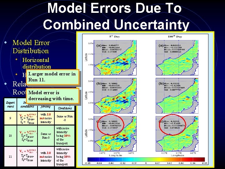
Model Errors Due To Combined Uncertainty • Model Error Distribution • Horizontal distribution Larger model error in • Histogram Run 11. • Relative Root Model Meanerror is decreasing with. Lateral time. Square Experi Initial Error Wind Boundary ment conditions forcing Conditions (RRMSE) 9 10 11 T 0 = TJD 180, S 0 = SJD 180 T 0=TJD 180, S 0=SJD 180 with 1. 0 m/s noise intensity Same as Run -0 Same as Run-0 with noise intensity being 10% of the transport with 1. 0 m/s noise intensity with noise intensity being 10% of the transport

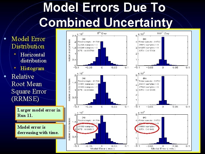
Model Errors Due To Combined Uncertainty • Model Error Distribution • Horizontal distribution • Histogram • Relative Root Mean Square Error (RRMSE) Larger model error in Run 11. Model error is decreasing with time.

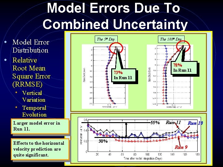
Model Errors Due To Combined Uncertainty • Model Error The 5 th Day Distribution • Relative Root Mean Square Error (RRMSE) The 180 th Day 78% In Run 11 73% In Run 11 • Vertical Variation • Temporal Evolution 55% Larger model error in Run 11. Effects to the horizontal velocity prediction are quite significant. Run 11 30% Run 9 Run 10

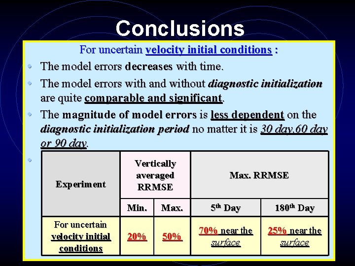
Conclusions For uncertain velocity initial conditions : • The model errors decreases with time. • The model errors with and without diagnostic initialization are quite comparable and significant. • The magnitude of model errors is less dependent on the diagnostic initialization period no matter it is 30 day, 60 day or 90 day. • Experiment For uncertain velocity initial conditions Vertically averaged RRMSE Max. RRMSE Min. Max. 5 th Day 180 th Day 20% 50% 70% near the surface 25% near the surface

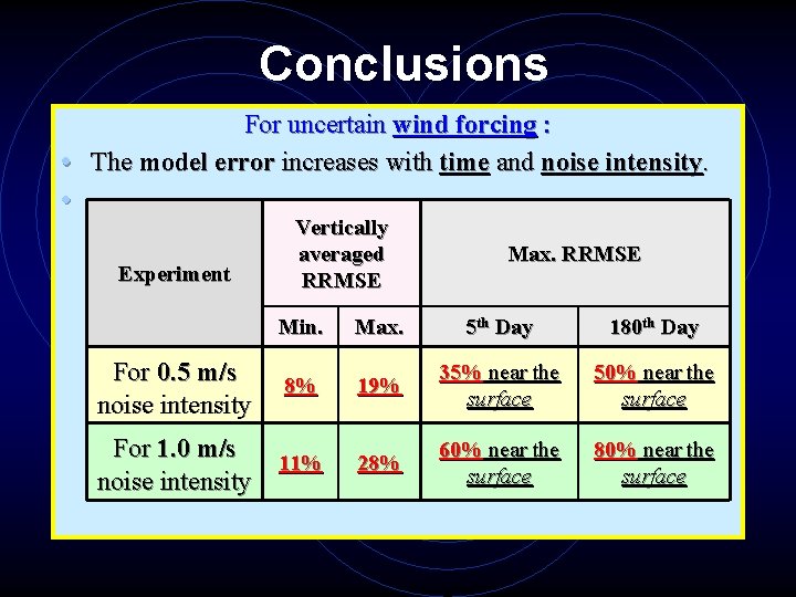
Conclusions For uncertain wind forcing : • The model error increases with time and noise intensity. • Experiment Vertically averaged RRMSE Max. RRMSE Min. Max. 5 th Day 180 th Day 8% 19% 35% near the surface 50% near the surface For 1. 0 m/s 11% noise intensity 28% 60% near the surface 80% near the surface For 0. 5 m/s noise intensity

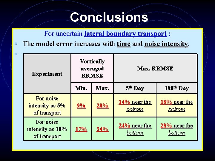
Conclusions For uncertain lateral boundary transport : • The model error increases with time and noise intensity. • Experiment Vertically averaged RRMSE Max. RRMSE Min. Max. 5 th Day 180 th Day For noise intensity as 5% of transport 9% 20% 14% near the bottom 18% near the bottom For noise intensity as 10% of transport 17% 34% 24% near the bottom 28% near the bottom

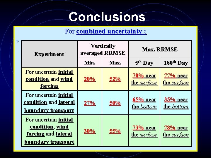
Conclusions For combined uncertainty : • Experiment Vertically averaged RRMSE Max. RRMSE 5 th Day 180 th Day Min. Max. For uncertain initial condition and wind forcing 20% 52% 70% near 77% near the surface For uncertain initial condition and lateral boundary transport 27% 50% 65% near the bottom For uncertain initial condition, wind forcing and lateral boundary transport 30% 55% 73% near 78% near the surface 35% near the bottom

? ? ? Question ?

Thank you !!