PREDICT 422 Practical Machine Learning Module 10 Unsupervised

PREDICT 422: Practical Machine Learning Module 10: Unsupervised Learning Lecturer: Nathan Bastian, Section: XXX

Assignment § Reading: Ch. 10 § Activity: Course Project

References § An Introduction to Statistical Learning, with Applications in R (2013), by G. James, D. Witten, T. Hastie, and R. Tibshirani. § The Elements of Statistical Learning (2009), by T. Hastie, R. Tibshirani, and J. Friedman. § Machine Learning: A Probabilistic Perspective (2012), by K. Murphy

Lesson Goals: § Understand principal components analysis for data visualization and dimension reduction. § Understand the K-means clustering algorithm. § Understand the hierarchical clustering algorithm.

Unsupervised Learning § Most of this course has focused on supervised learning methods such as regression and classification. § Remember that in supervised learning we observe both a set of features as well as a response (or outcome variable). § In unsupervised learning, however, we only observe features. We are not interested in prediction because we do not have an associated response variable. § The goal is to discover interesting things about the measurements.

Unsupervised Learning (cont’d) § Here, we discuss two methods: – Principal Components Analysis: a tool used for data visualization or data preprocessing before supervised techniques are applied. – Clustering: a broad class of methods for discovering unknown subgroups in data. § Unsupervised learning is more subjective than supervised learning, as there is no simple goal for the analysis (such as prediction of a response). § Applications: – Subgroups of breast cancer patients groups by their gene expression measurements. – Groups of shoppers characterized by their browsing and purchase histories. – Movies grouped by the ratings assigned by movie viewers.

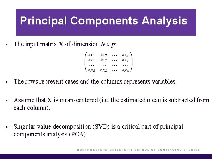
Principal Components Analysis § The input matrix X of dimension N x p: § The rows represent cases and the columns represents variables. § Assume that X is mean-centered (i. e. the estimated mean is subtracted from each column). § Singular value decomposition (SVD) is a critical part of principal components analysis (PCA).

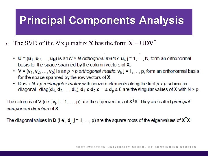
Principal Components Analysis § The SVD of the N x p matrix X has the form X = UDVT

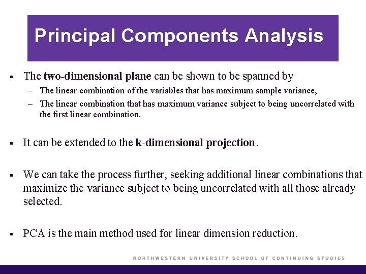
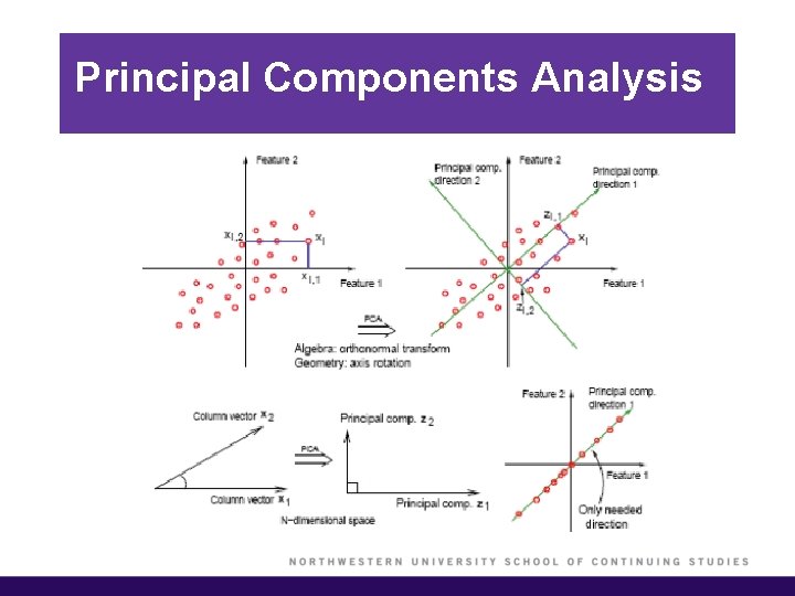
Principal Components Analysis § The two-dimensional plane can be shown to be spanned by – The linear combination of the variables that has maximum sample variance, – The linear combination that has maximum variance subject to being uncorrelated with the first linear combination. § It can be extended to the k-dimensional projection. § We can take the process further, seeking additional linear combinations that maximize the variance subject to being uncorrelated with all those already selected. § PCA is the main method used for linear dimension reduction.

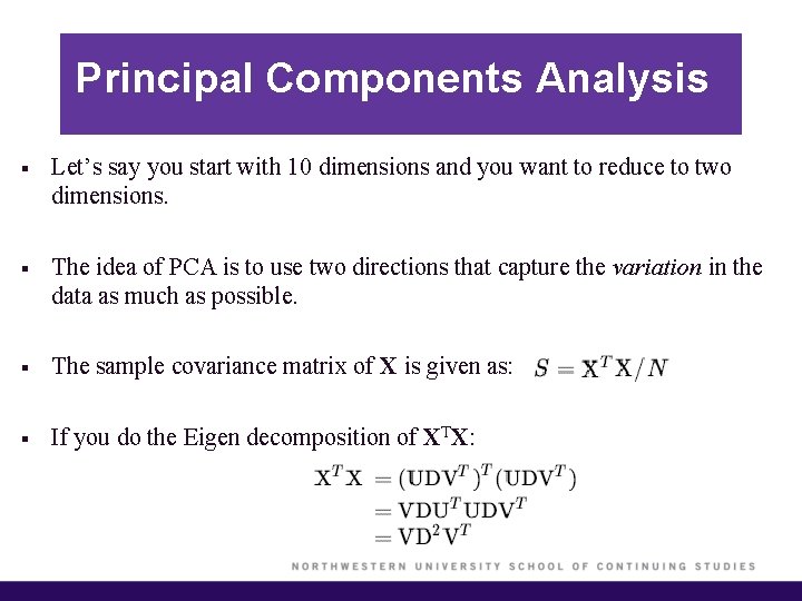
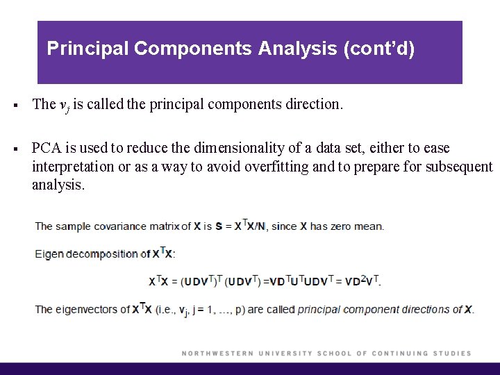
Principal Components Analysis § Let’s say you start with 10 dimensions and you want to reduce to two dimensions. § The idea of PCA is to use two directions that capture the variation in the data as much as possible. § The sample covariance matrix of X is given as: § If you do the Eigen decomposition of XTX:

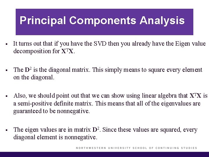
Principal Components Analysis § It turns out that if you have the SVD then you already have the Eigen value decomposition for XTX. § The D 2 is the diagonal matrix. This simply means to square every element on the diagonal. § Also, we should point out that we can show using linear algebra that XTX is a semi-positive definite matrix. This means that all of the eigenvalues are guaranteed to be nonnegative. § The eigen values are in matrix D 2. Since these values are squared, every diagonal element is nonnegative.

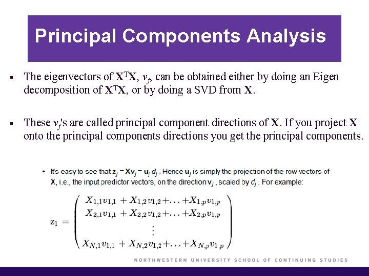
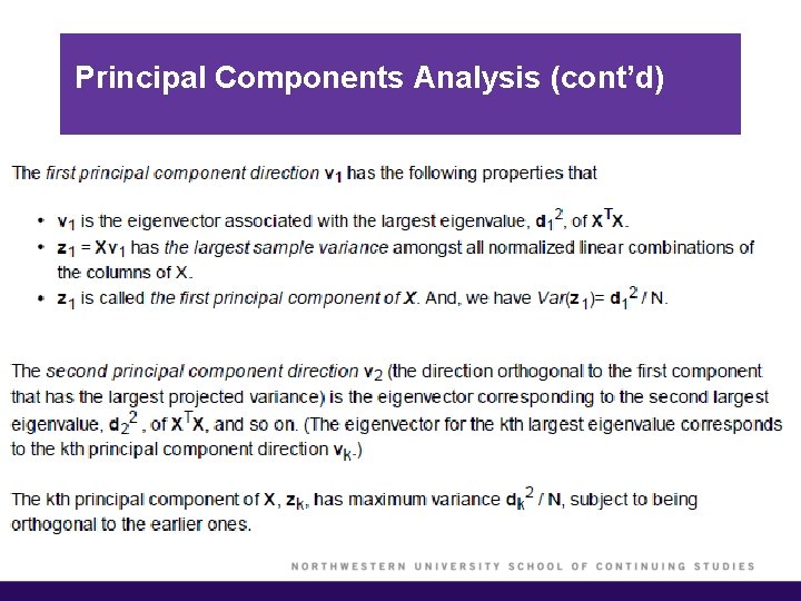
Principal Components Analysis § The eigenvectors of XTX, vj, can be obtained either by doing an Eigen decomposition of XTX, or by doing a SVD from X. § These vj's are called principal component directions of X. If you project X onto the principal components directions you get the principal components.

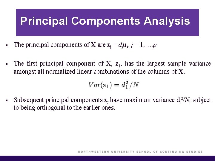
Principal Components Analysis § The principal components of X are zj = djuj, j = 1, …, p § The first principal component of X, z 1, has the largest sample variance amongst all normalized linear combinations of the columns of X. § Subsequent principal components zj have maximum variance dj 2/N, subject to being orthogonal to the earlier ones.

Principal Components Analysis

Principal Components Analysis § Why are we interested in this? Consider an extreme case, where your data all lie in one direction. § Although two features represent the data, we can reduce the dimension of the dataset to one using a single linear combination of the features (as given by the first principal component). § Just to summarize the way you do dimension reduction. First you have X, and you remove the means. On X you do a singular value decomposition and obtain matrices U, D, and V. § Then you call every column vector in V, vj, where j = 1, . . . , p.

Principal Components Analysis (cont’d) § The vj is called the principal components direction. § PCA is used to reduce the dimensionality of a data set, either to ease interpretation or as a way to avoid overfitting and to prepare for subsequent analysis.

Principal Components Analysis (cont’d)

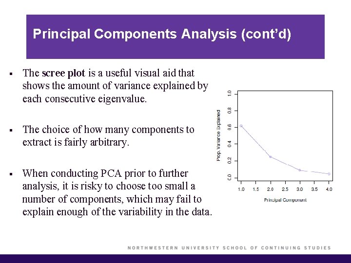
Principal Components Analysis (cont’d) § The scree plot is a useful visual aid that shows the amount of variance explained by each consecutive eigenvalue. § The choice of how many components to extract is fairly arbitrary. § When conducting PCA prior to further analysis, it is risky to choose too small a number of components, which may fail to explain enough of the variability in the data.

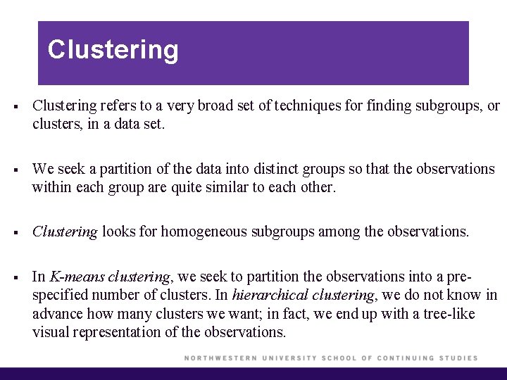
Clustering § Clustering refers to a very broad set of techniques for finding subgroups, or clusters, in a data set. § We seek a partition of the data into distinct groups so that the observations within each group are quite similar to each other. § Clustering looks for homogeneous subgroups among the observations. § In K-means clustering, we seek to partition the observations into a prespecified number of clusters. In hierarchical clustering, we do not know in advance how many clusters we want; in fact, we end up with a tree-like visual representation of the observations.

Clustering (cont’d)

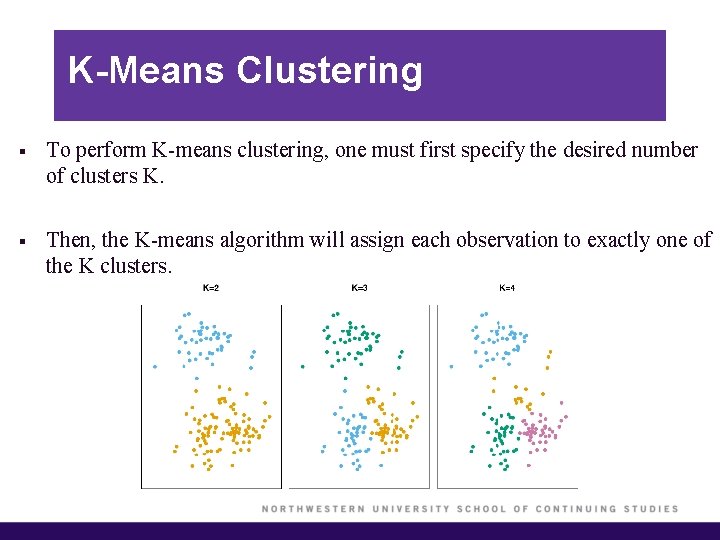
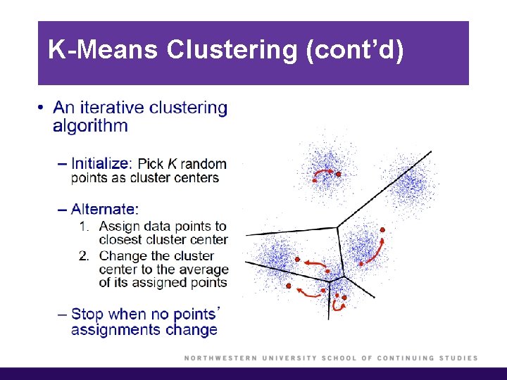
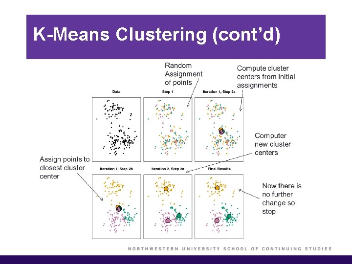
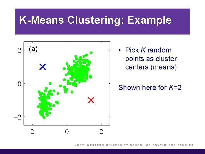
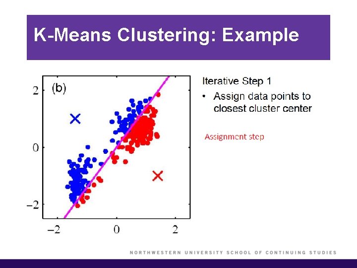
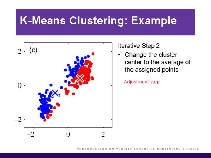
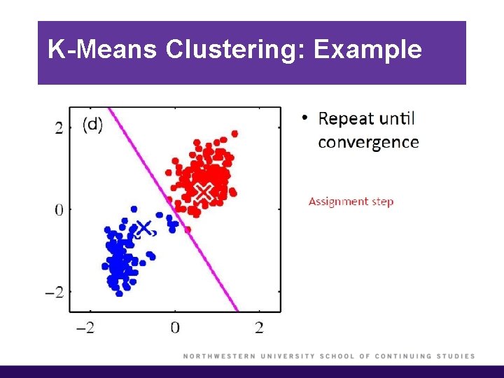
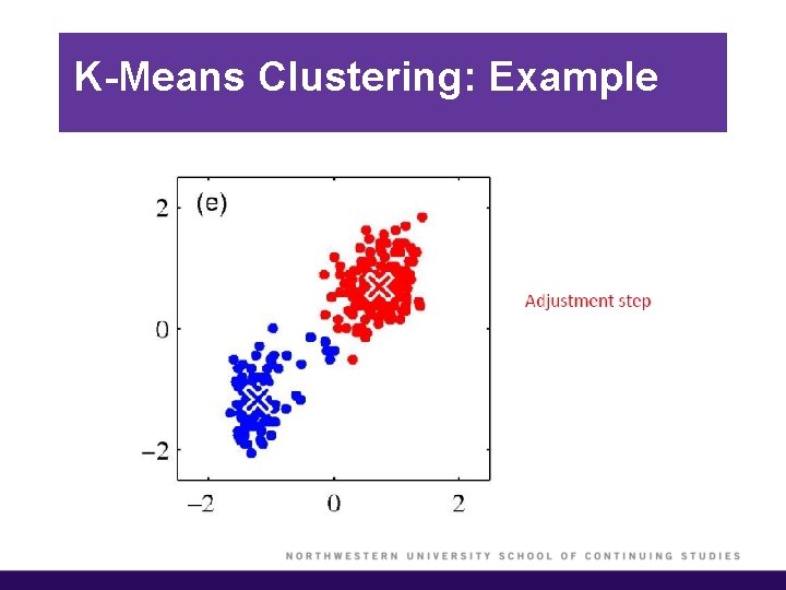
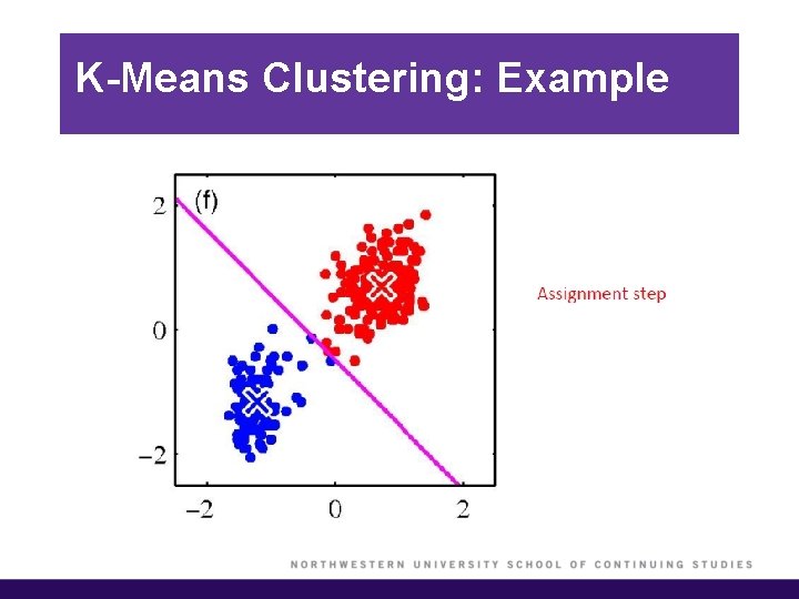
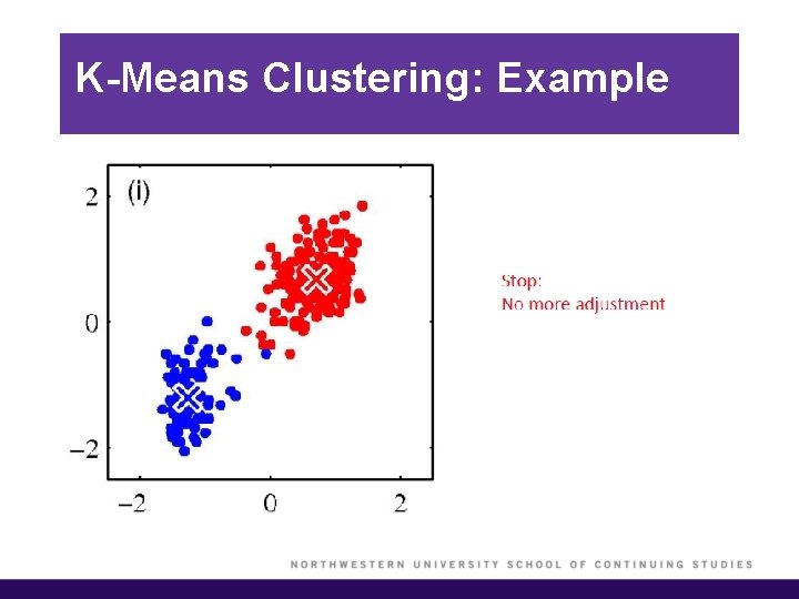
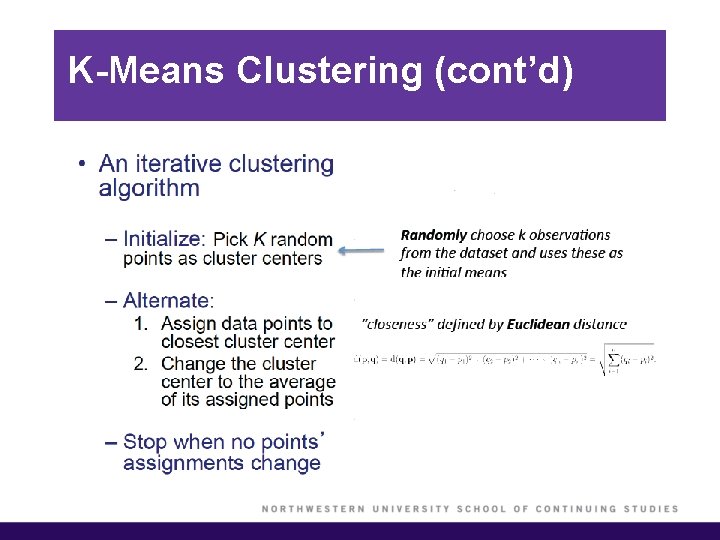
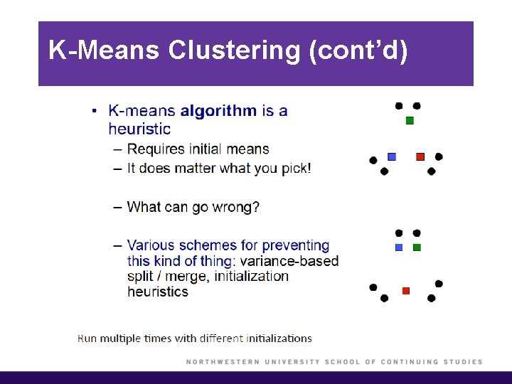
K-Means Clustering § To perform K-means clustering, one must first specify the desired number of clusters K. § Then, the K-means algorithm will assign each observation to exactly one of the K clusters.

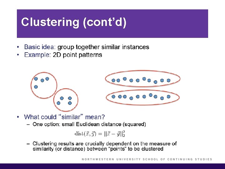
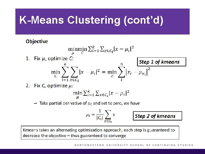
K-Means Clustering (cont’d) § We would like to partition the data set into K clusters, where each observation belongs to at least one of the K clusters. § The clusters are non-overlapping, i. e. no observation belongs to more than one cluster. § The objective is to have a minimal “within-cluster-variation”, i. e. the elements within a cluster should be as similar as possible. § One way of achieving this is to minimize the sum of all the pair-wise squared Euclidean distances between the observations in each cluster.

K-Means Clustering (cont’d)

K-Means Clustering (cont’d)

K-Means Clustering: Example

K-Means Clustering: Example

K-Means Clustering: Example

K-Means Clustering: Example

K-Means Clustering: Example

K-Means Clustering: Example

K-Means Clustering: Example

K-Means Clustering (cont’d)

K-Means Clustering (cont’d)

K-Means Clustering (cont’d)

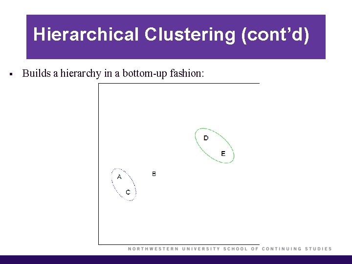
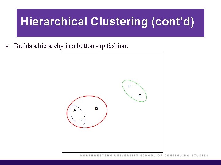
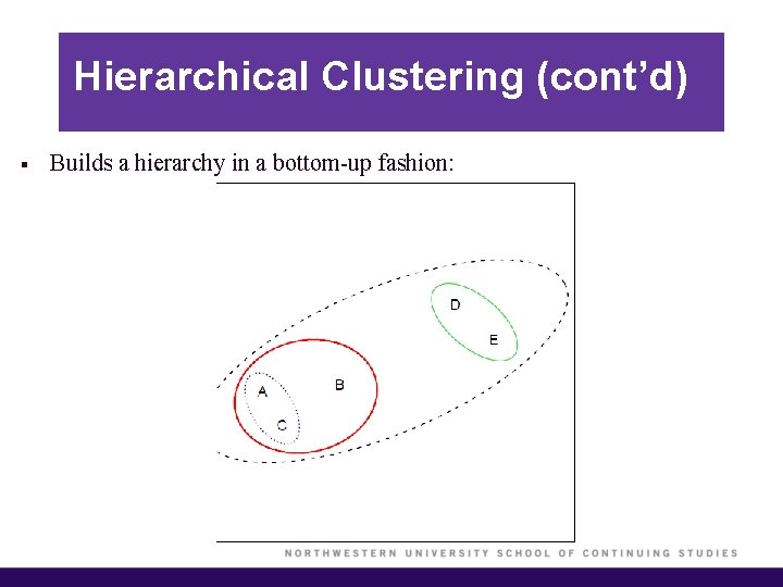
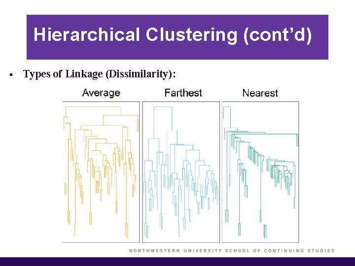
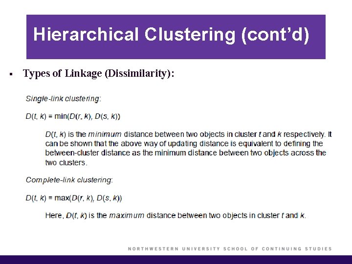
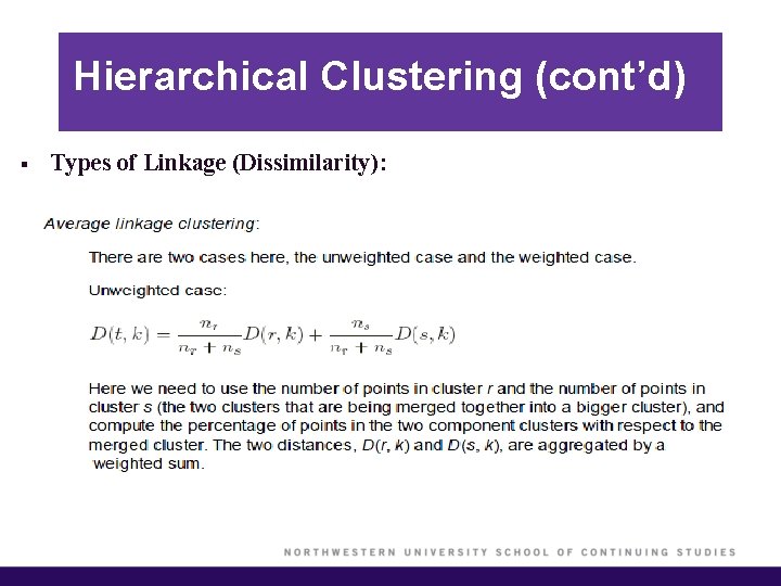
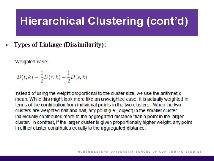
Hierarchical Clustering § K-means clustering requires choosing the number of clusters. If we don’t want to do that, an alternative is to use hierarchical clustering. § Hierarchical clustering has an added advantage that it produces a tree-based representation of the observations, called a dendrogram. § The most common type of hierarchical clustering is called agglomerative clustering (or bottom-up), which refers to the fact that a dendrogram is built starting from the leaves and combining clusters up to the trunk. § Agglomerative clustering can be used as long as we have pairwise distances between any two objects.

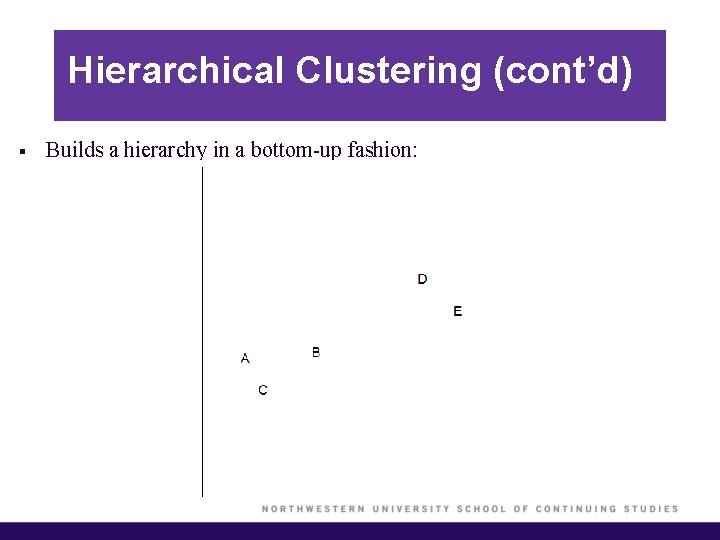
Hierarchical Clustering (cont’d) § Builds a hierarchy in a bottom-up fashion:

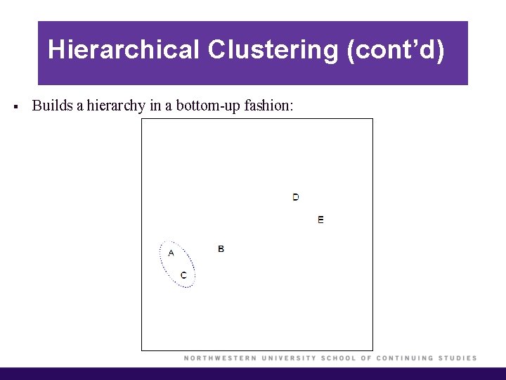
Hierarchical Clustering (cont’d) § Builds a hierarchy in a bottom-up fashion:

Hierarchical Clustering (cont’d) § Builds a hierarchy in a bottom-up fashion:

Hierarchical Clustering (cont’d) § Builds a hierarchy in a bottom-up fashion:

Hierarchical Clustering (cont’d) § Builds a hierarchy in a bottom-up fashion:

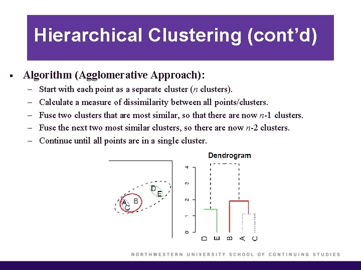
Hierarchical Clustering (cont’d) § Algorithm (Agglomerative Approach): – – – Start with each point as a separate cluster (n clusters). Calculate a measure of dissimilarity between all points/clusters. Fuse two clusters that are most similar, so that there are now n-1 clusters. Fuse the next two most similar clusters, so there are now n-2 clusters. Continue until all points are in a single cluster.

Hierarchical Clustering (cont’d) § Each “leaf” of the dendrogram represents one of the observations. § At the bottom of the dendrogram, each observation is a distinct leaf. However, as we move up the tree, some leaves begin to fuse. These correspond to observations that are similar to each other. § As we move higher up the tree, an increasing number of observations have fused. The earlier (lower in the tree) two observations fuse, the more similar they are to each other. § Observations that fuse later are quite different.

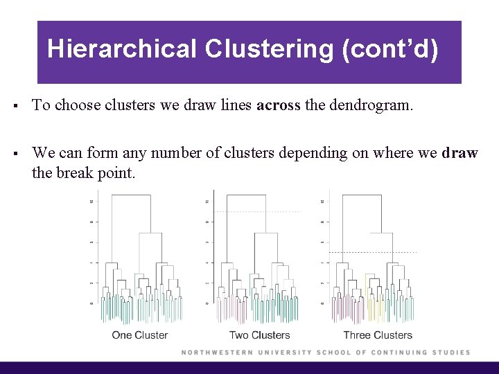
Hierarchical Clustering (cont’d) § To choose clusters we draw lines across the dendrogram. § We can form any number of clusters depending on where we draw the break point.

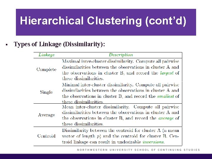
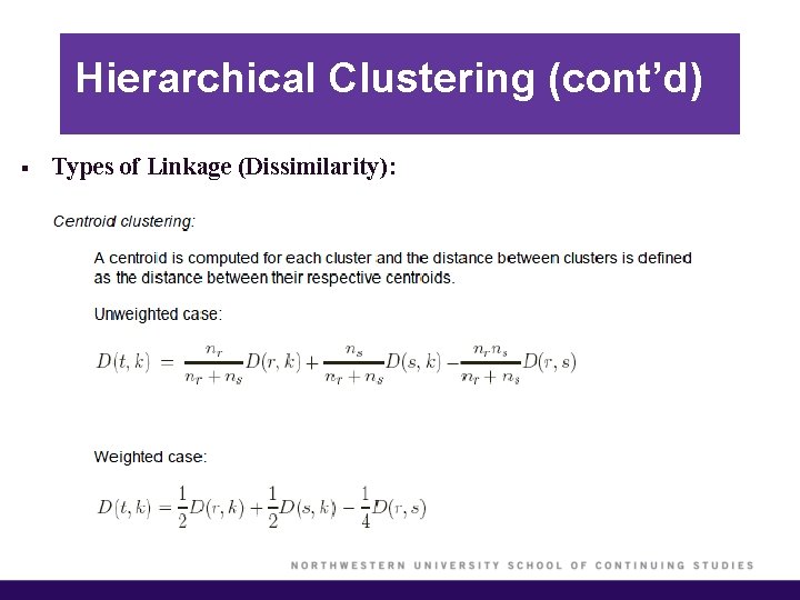
Hierarchical Clustering (cont’d) § Types of Linkage (Dissimilarity):

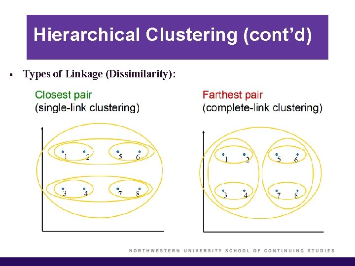
Hierarchical Clustering (cont’d) § Types of Linkage (Dissimilarity):

Hierarchical Clustering (cont’d) § Types of Linkage (Dissimilarity):

Hierarchical Clustering (cont’d) § Types of Linkage (Dissimilarity):

Hierarchical Clustering (cont’d) § Types of Linkage (Dissimilarity):

Hierarchical Clustering (cont’d) § Types of Linkage (Dissimilarity):

Hierarchical Clustering (cont’d) § Types of Linkage (Dissimilarity):

Summary § PCA for data visualization and dimension reduction. § K-means clustering algorithm. § Hierarchical clustering algorithm.