PREDATORPREY CELLULAR AUTOMATA Richard Peters ES 314 Sonoma

PREDATOR/PREY CELLULAR AUTOMATA Richard Peters ES 314 Sonoma State University

Cellular Automata • “A cellular automaton is a collection of "colored" cells on a grid of specified shape that evolves through a number of discrete time steps according to a set of rules based on the states of neighboring cells. The rules are then applied iteratively for as many time steps as desired. ” – Weisstein, Eric W. "Cellular Automaton. " From Math. World--A Wolfram Web Resource. http: //mathworld. wolfram. com/Cellular. Automato n. html

Basic Idea • Generate an Nx. N grid. • Create two species of cellular automata: predator and prey on the grid. • Provide a set of rules for behavior of each species. • If a predator automaton ‘catches’ a prey automaton – the prey is ‘killed’.

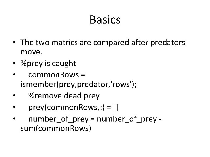
Basics • Automata are merely grid cells. Each species comprises an Nx 2 matrix denoting its position. Each automata is assigned a color according to its specifies type. • Motion is implemented by generating a random number 1 -8 where each number represents the next direction to move.

Basics • The two matrics are compared after predators move. • %prey is caught • common. Rows = ismember(prey, predator, 'rows'); • %remove dead prey • prey(common. Rows, : ) = [] • number_of_prey = number_of_prey sum(common. Rows)

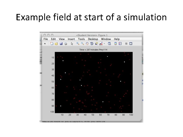
Example field at start of a simulation

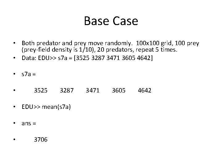
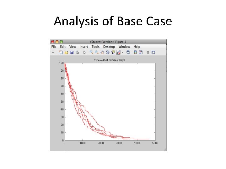
Base Case • Both predator and prey move randomly. 100 x 100 grid, 100 prey (prey-field density is 1/10), 20 predators, repeat 5 times. • Data: EDU>> s 7 a = [3525 3287 3471 3605 4642] • s 7 a = • 3525 3287 • EDU>> mean(s 7 a) • ans = • 3706 3471 3605 4642

Analysis of Base Case

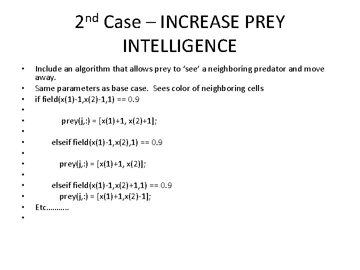
2 nd Case – INCREASE PREY INTELLIGENCE • • • • Include an algorithm that allows prey to ‘see’ a neighboring predator and move away. Same parameters as base case. Sees color of neighboring cells if field(x(1)-1, x(2)-1, 1) == 0. 9 prey(j, : ) = [x(1)+1, x(2)+1]; elseif field(x(1)-1, x(2), 1) == 0. 9 prey(j, : ) = [x(1)+1, x(2)]; elseif field(x(1)-1, x(2)+1, 1) == 0. 9 prey(j, : ) = [x(1)+1, x(2)-1]; Etc………. .

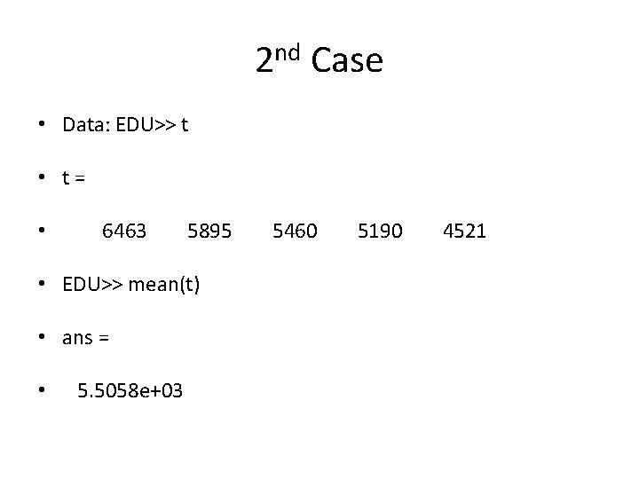
2 nd Case • Data: EDU>> t • t= • 6463 5895 • EDU>> mean(t) • ans = • 5. 5058 e+03 5460 5190 4521

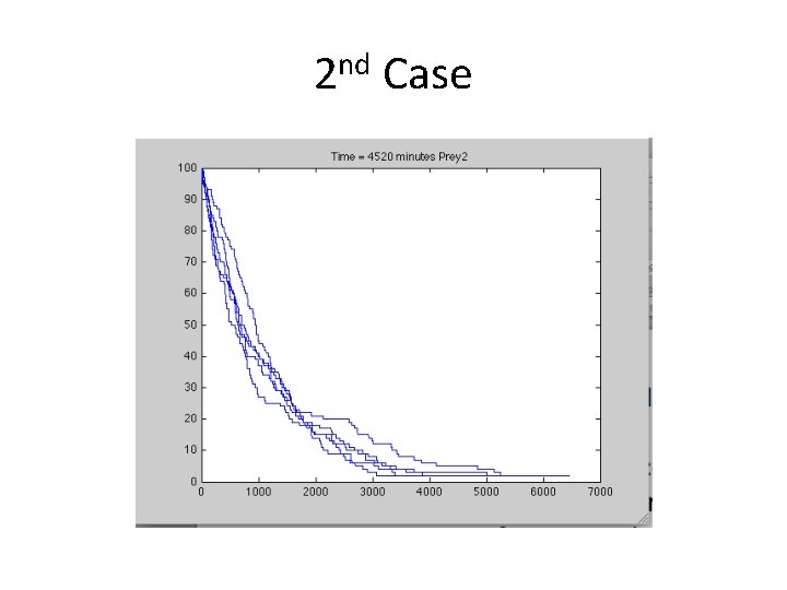
2 nd Case

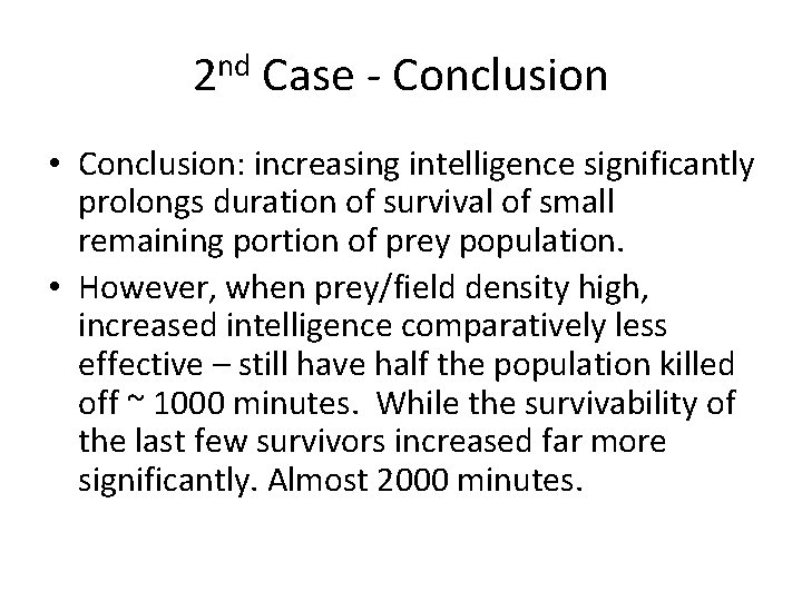
2 nd Case - Conclusion • Conclusion: increasing intelligence significantly prolongs duration of survival of small remaining portion of prey population. • However, when prey/field density high, increased intelligence comparatively less effective – still have half the population killed off ~ 1000 minutes. While the survivability of the last few survivors increased far more significantly. Almost 2000 minutes.

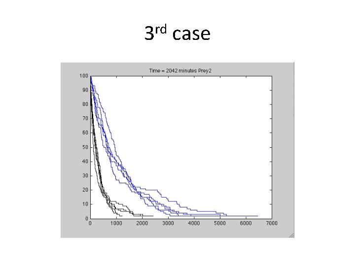
3 rd – Smarter Predators • Remove ‘sight’ algorithm from Prey automata and insert in Predator automata. • t= • 2434 1126 • EDU>> mean(t) • ans = • 1. 7858 e+03 2094 1232 2043

3 rd case

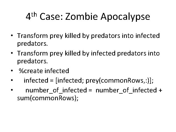
4 th Case: Zombie Apocalypse • Transform prey killed by predators into infected predators. • Transform prey killed by infected predators into predators. • %create infected • infected = [infected; prey(common. Rows, : )]; • number_of_infected = number_of_infected + sum(common. Rows);

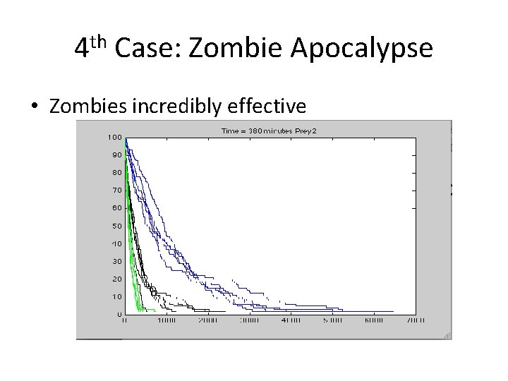
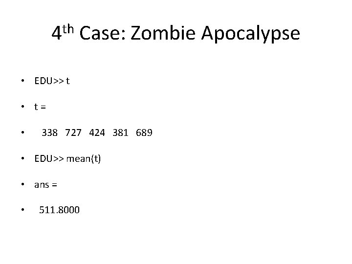
4 th Case: Zombie Apocalypse • Zombies incredibly effective

4 th Case: Zombie Apocalypse • EDU>> t • t= • 338 727 424 381 689 • EDU>> mean(t) • ans = • 511. 8000

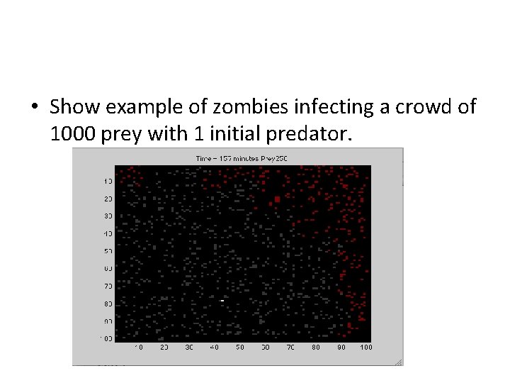
• Show example of zombies infecting a crowd of 1000 prey with 1 initial predator.

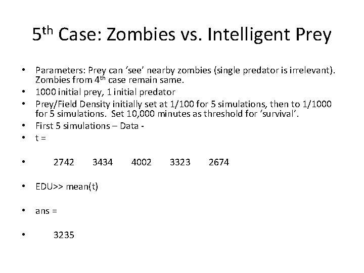
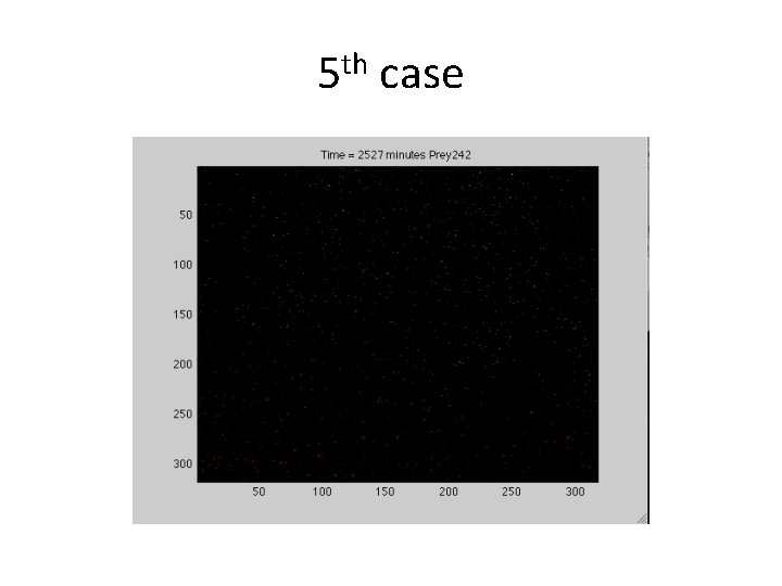
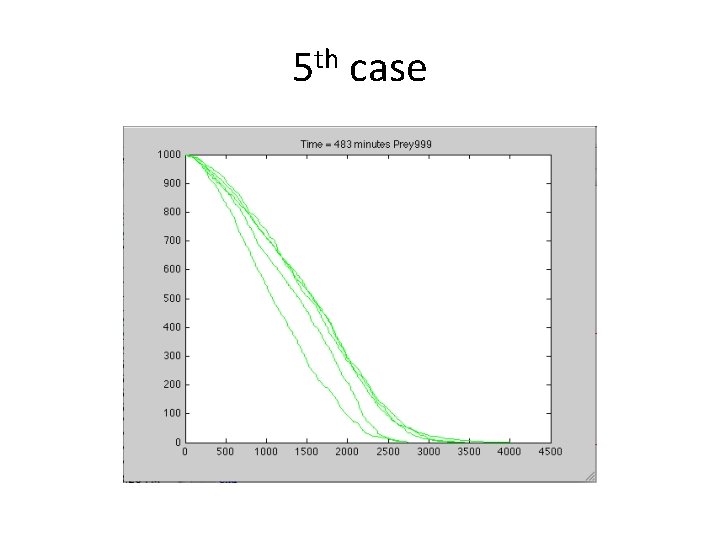
5 th Case: Zombies vs. Intelligent Prey • Parameters: Prey can ‘see’ nearby zombies (single predator is irrelevant). Zombies from 4 th case remain same. • 1000 initial prey, 1 initial predator • Prey/Field Density initially set at 1/100 for 5 simulations, then to 1/1000 for 5 simulations. Set 10, 000 minutes as threshold for ‘survival’. • First 5 simulations – Data • t= • 2742 3434 • EDU>> mean(t) • ans = • 3235 4002 3323 2674

5 th case

5 th case

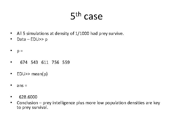
5 th case • All 5 simulations at density of 1/1000 had prey survive. • Data – EDU>> p • p= • 674 543 611 756 559 • EDU>> mean(p) • ans = • 628. 6000 • Conclusion – prey intelligence plus more low population densities are key to prey survival.

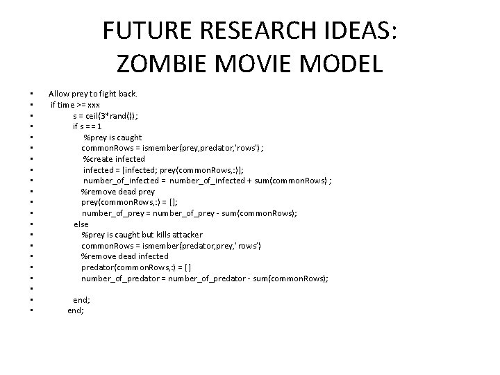
FUTURE RESEARCH IDEAS: ZOMBIE MOVIE MODEL • • • • • • Allow prey to fight back. if time >= xxx s = ceil(3*rand()) ; if s == 1 %prey is caught common. Rows = ismember(prey, predator, 'rows') ; %create infected = [infected; prey(common. Rows, : )]; number_of_infected = number_of_infected + sum(common. Rows) ; %remove dead prey(common. Rows, : ) = []; number_of_prey = number_of_prey - sum(common. Rows); else %prey is caught but kills attacker common. Rows = ismember(predator, prey, ' rows’) %remove dead infected predator(common. Rows, : ) = [ ] number_of_predator = number_of_predator - sum(common. Rows); end;

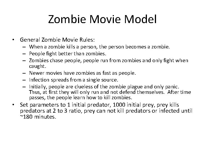
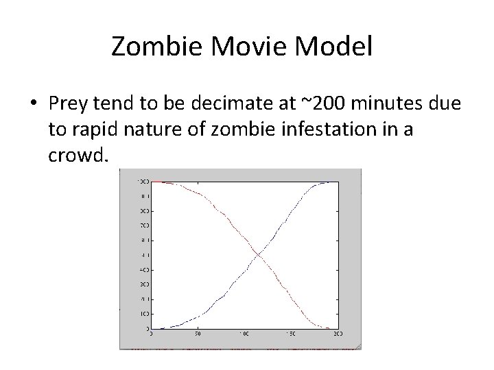
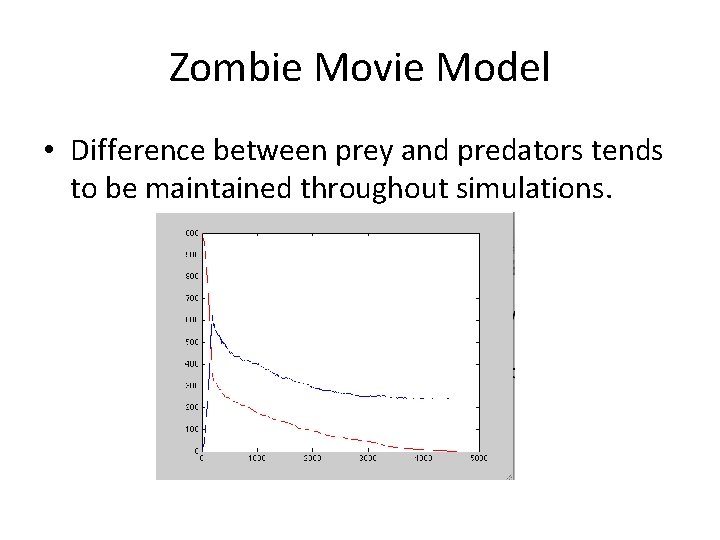
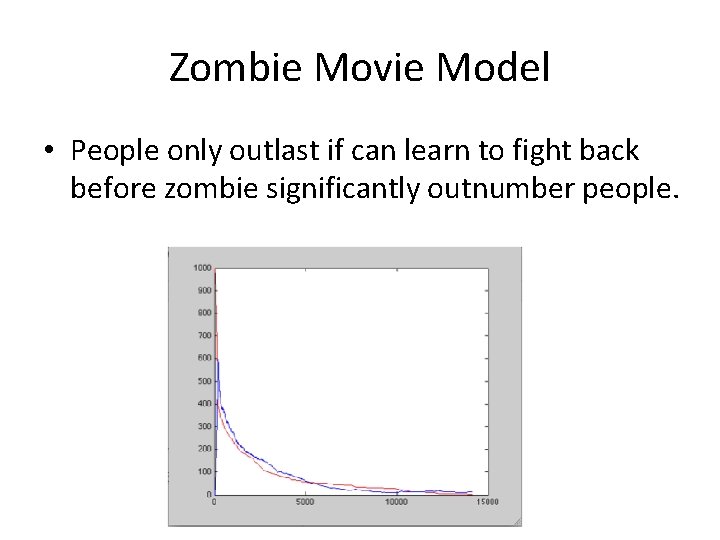
Zombie Movie Model • General Zombie Movie Rules: – When a zombie kills a person, the person becomes a zombie. – People fight better than zombies. – Zombies chase people, people run from zombies and only fight when caught. – Newer movies have zombies as fast as people. – Infection spreads from a single source. – Initially, people are clueless of the zombie plague and only panic. Thus, at first they will only run and not defend themselves. After time passes, the people learn how to kill zombies. • Set parameters to 1 initial predator, 1000 initial prey, prey kills predators at 2 to 3 ratio, prey can not kill predators or infected until ~180 minutes.

Zombie Movie Model • Prey tend to be decimate at ~200 minutes due to rapid nature of zombie infestation in a crowd.

Zombie Movie Model • Difference between prey and predators tends to be maintained throughout simulations.

Zombie Movie Model • People only outlast if can learn to fight back before zombie significantly outnumber people.

Other potential simulation attributes • Additional attributes that can be added – Prey can have a herding instinct. – Increase distance components can see. – Increase prey fighting abilities with fighting experience. – Add barriers to field that simulate urban environment.

TAKE AWAY • If you find yourself in a zombie apocalypse, stay away from crowds and cities.