Predator Prey Systems with an Alternative Food Source

Predator Prey Systems with an Alternative Food Source By Karuna Batcha and Victoria Nicolov

Introduction § Extension Of Lotka-Volterra § Realistic Application of the model § Question: Under what conditions is stability likely to occur because of food source switching? § Results: Differed significantly from Lotka Volterra, and adjustments to parameters lead to various long term solutions.

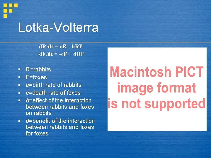
Lotka-Volterra d. R/dt = a. R - b. RF d. F/dt = -c. F + d. RF § § § R=rabbits F=foxes a=birth rate of rabbits c=death rate of foxes b=effect of the interaction between rabbits and foxes on rabbits § d=benefit of the interaction between rabbits and foxes for foxes

Geometric Representation

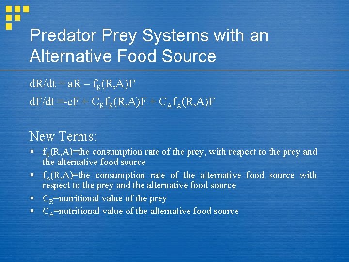
Predator Prey Systems with an Alternative Food Source d. R/dt = a. R – f. R(R, A)F d. F/dt =-c. F + CRf. R(R, A)F + CAf. A(R, A)F New Terms: § f. R(R, A)=the consumption rate of the prey, with respect to the prey and the alternative food source § f. A(R, A)=the consumption rate of the alternative food source with respect to the prey and the alternative food source § CR=nutritional value of the prey § CA=nutritional value of the alternative food source

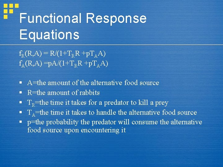
Functional Response Equations f. R(R, A) = R/(1+TRR +p. TAA) f. A(R, A) =p. A/(1+TRR +p. TAA) § § § A=the amount of the alternative food source R=the amount of rabbits TR=the time it takes for a predator to kill a prey TA=the time it takes to handle the alternative food source p=the probability the predator will consume the alternative food source upon encountering it

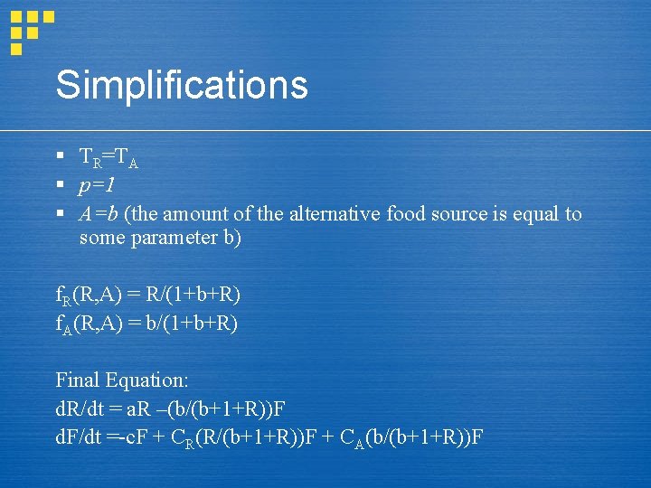
Simplifications § TR=TA § p=1 § A=b (the amount of the alternative food source is equal to some parameter b) f. R(R, A) = R/(1+b+R) f. A(R, A) = b/(1+b+R) Final Equation: d. R/dt = a. R –(b/(b+1+R))F d. F/dt =-c. F + CR(R/(b+1+R))F + CA(b/(b+1+R))F

Example 1 § § a=3 c=1 CR=CA=1 b=1 d. R/dt = 3 R –(1/(1+1+R))F d. F/dt =-1 F + 1(R/(1+1+R))F +1(1/(1+1+R))F

Example § § § a=3 c=1 CR=1 CA=5 b=1 2 d. R/dt = 3 R –(1/(1+1+R))F d. F/dt =-1 F + 1(R/(1+1+R))F + 5(1(1+1+R))F

Example 3 d. R/dt = a. R –(b/(b+1+R))F d. F/dt =-c. F + CR(R/(b+1+R))F + CA(b/(b+1+R))F § § § a=3 c=1 CR=3 CA=1 b=1

Conclusion § Nutritional values drastically changed the system § No stable equilibrium (except (0, 0)) § Nullclines predicted the appearance of the graphs