PRAM architectures algorithms performance evaluation 1 Shared Memory

PRAM architectures, algorithms, performance evaluation 1

Shared Memory model and PRAM • p processors, each may have local memory – Each processor has index, available to local code • Shared memory • During each time unit, each processor either – Performs one compute operation, or – Performs one memory access • Challenging. Means very good shared memory (maybe small) • Two modes: – Synchronous: all processors use same clock (PRAM) – Asynchronous: synchronization is code responsibility • Asynchronous is more realistic 2

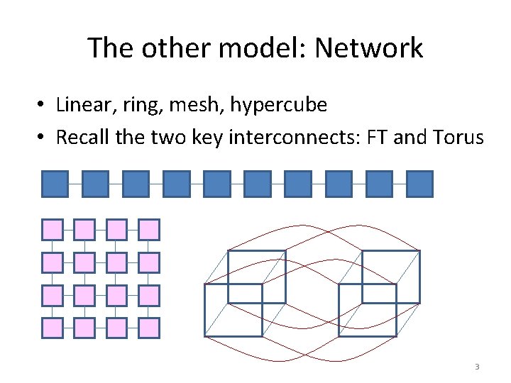
The other model: Network • Linear, ring, mesh, hypercube • Recall the two key interconnects: FT and Torus 3

A first glimpse, based on • Joseph F. Ja, Introduction to Parallel Algorithms, 1992 – www. umiacs. umd. edu/~joseph/ • Uzi Vishkin, PRAM concepts (1981 -today) – www. umiacs. umd. edu/~vishkin 4

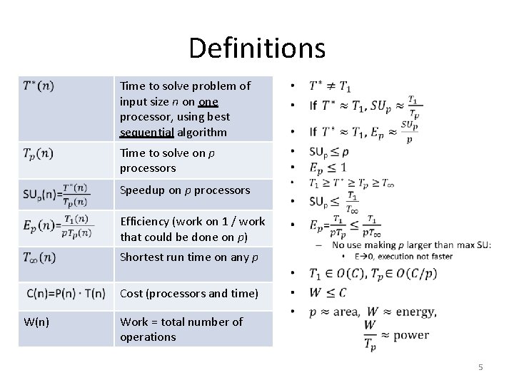
Definitions Time to solve problem of input size n on one processor, using best sequential algorithm • Time to solve on p processors Speedup on p processors Efficiency (work on 1 / work that could be done on p) Shortest run time on any p Cost (processors and time) W(n) Work = total number of operations 5

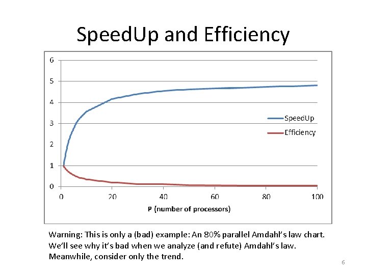
Speed. Up and Efficiency Warning: This is only a (bad) example: An 80% parallel Amdahl’s law chart. We’ll see why it’s bad when we analyze (and refute) Amdahl’s law. Meanwhile, consider only the trend. 6

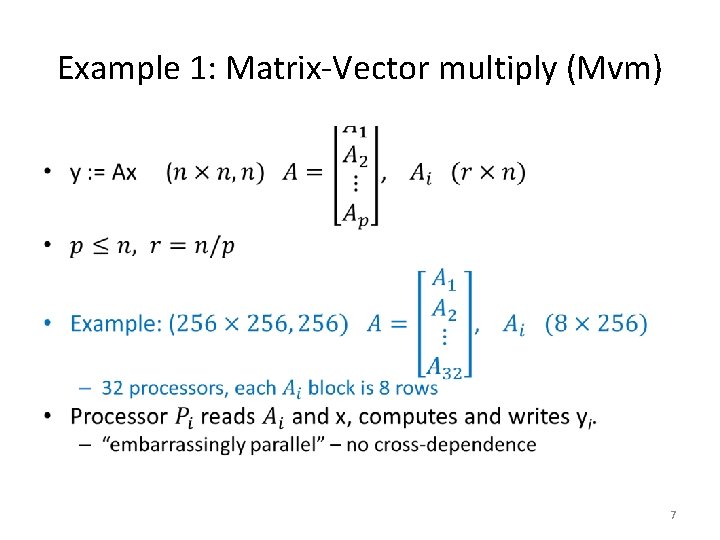
Example 1: Matrix-Vector multiply (Mvm) • 7

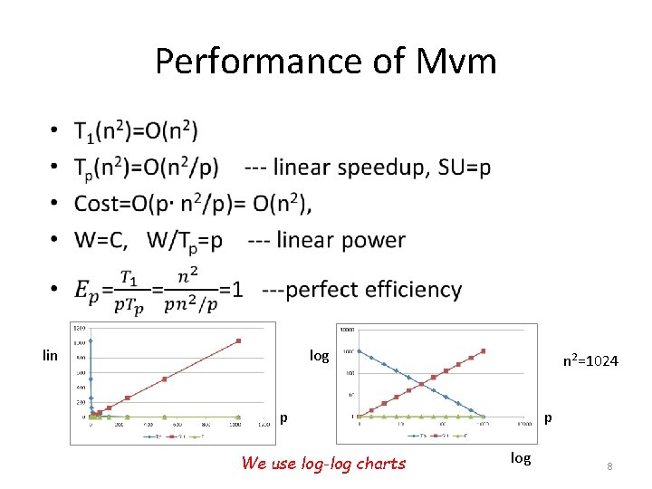
Performance of Mvm • lin log n 2=1024 p We use log-log charts p log 8

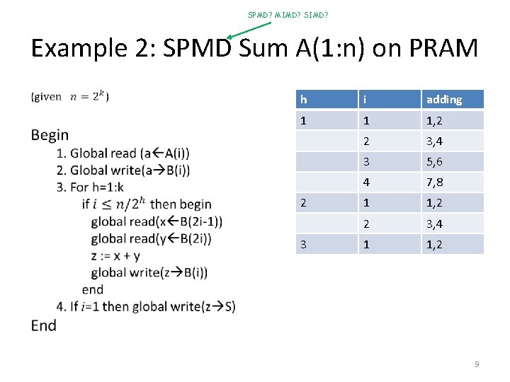
SPMD? MIMD? SIMD? Example 2: SPMD Sum A(1: n) on PRAM • h i adding 1 1 1, 2 2 3, 4 3 5, 6 4 7, 8 1 1, 2 2 3, 4 1 1, 2 2 3 9

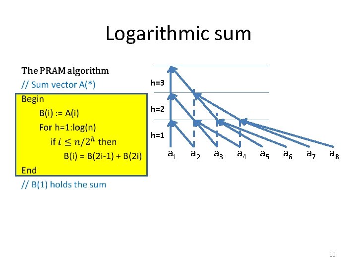
Logarithmic sum • h=3 h=2 h=1 a 2 a 3 a 4 a 5 a 6 a 7 a 8 10

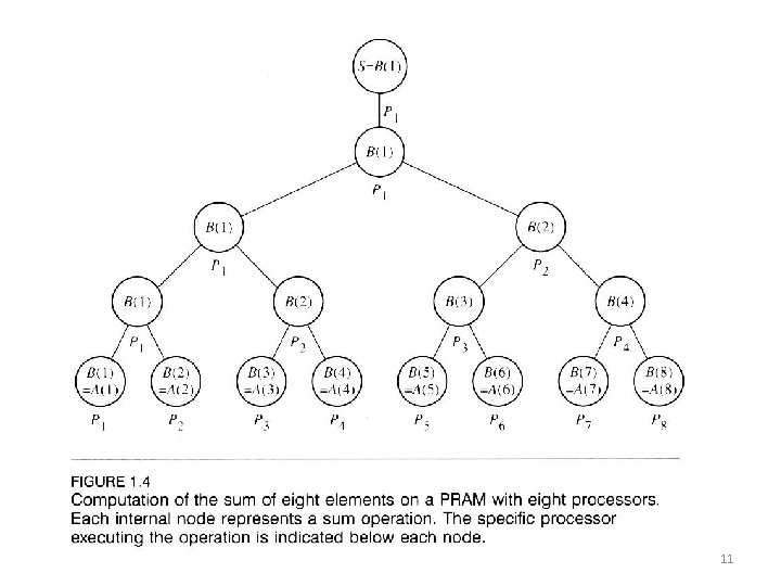
11

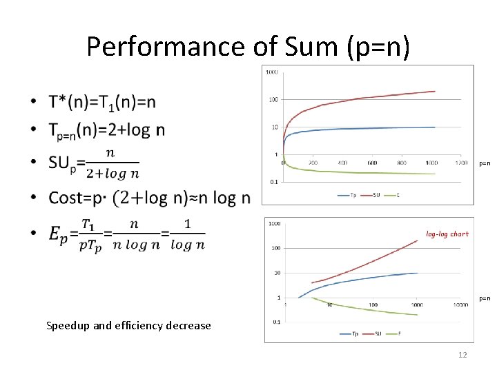
Performance of Sum (p=n) • p=n log-log chart p=n Speedup and efficiency decrease 12

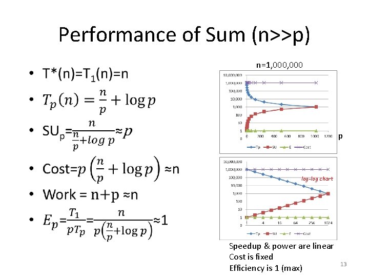
Performance of Sum (n>>p) • n=1, 000 p log-log chart Speedup & power are linear Cost is fixed Efficiency is 1 (max) 13

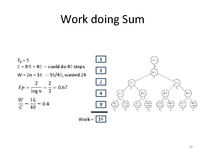
Work doing Sum T 8 = 5 C = 8 5 = 40 -- could do 40 steps W = 2 n = 16 -- 16/40, wasted 24 1 1 2 4 8 Work = 16 14

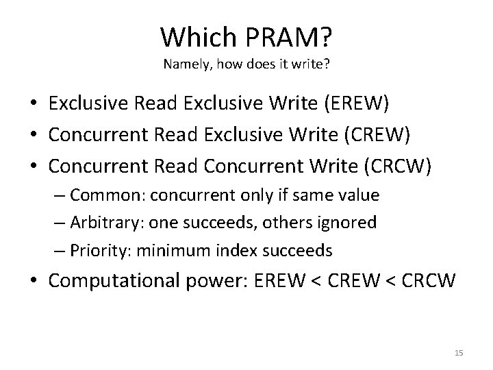
Which PRAM? Namely, how does it write? • Exclusive Read Exclusive Write (EREW) • Concurrent Read Exclusive Write (CREW) • Concurrent Read Concurrent Write (CRCW) – Common: concurrent only if same value – Arbitrary: one succeeds, others ignored – Priority: minimum index succeeds • Computational power: EREW < CRCW 15

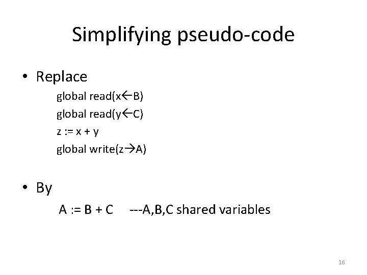
Simplifying pseudo-code • Replace global read(x B) global read(y C) z : = x + y global write(z A) • By A : = B + C ---A, B, C shared variables 16

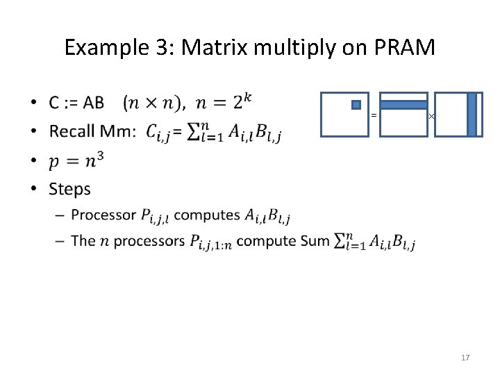
Example 3: Matrix multiply on PRAM • = × 17

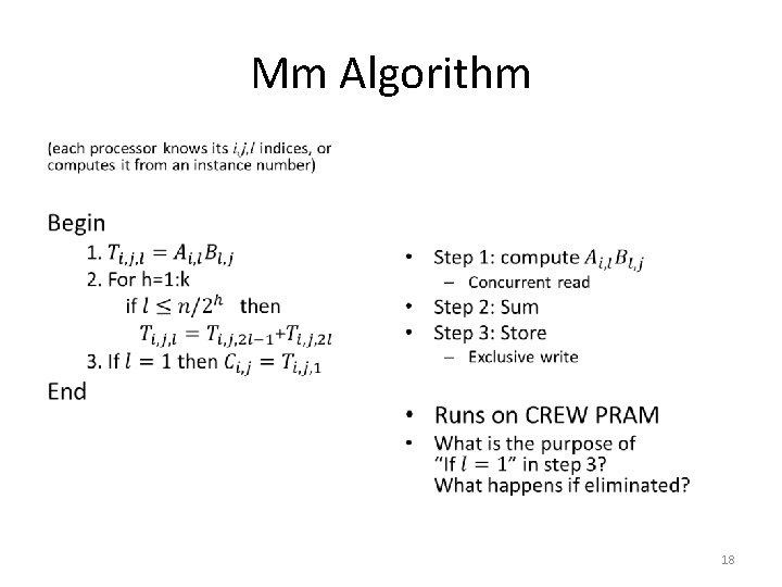
Mm Algorithm • • 18

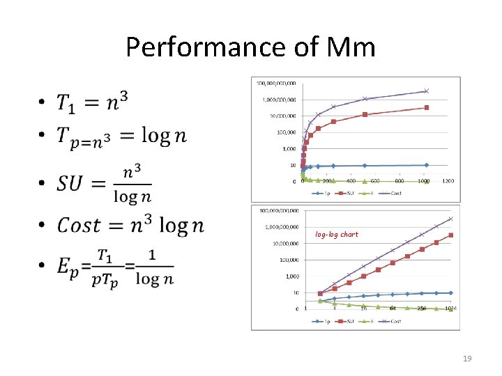
Performance of Mm • log-log chart 19

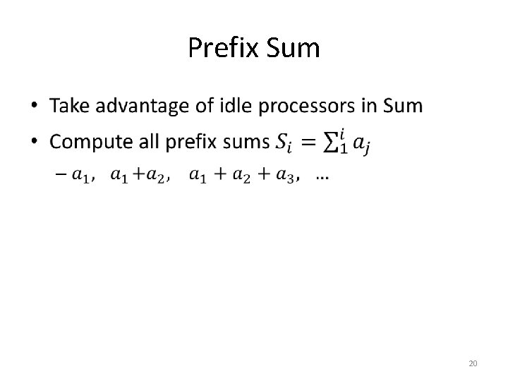
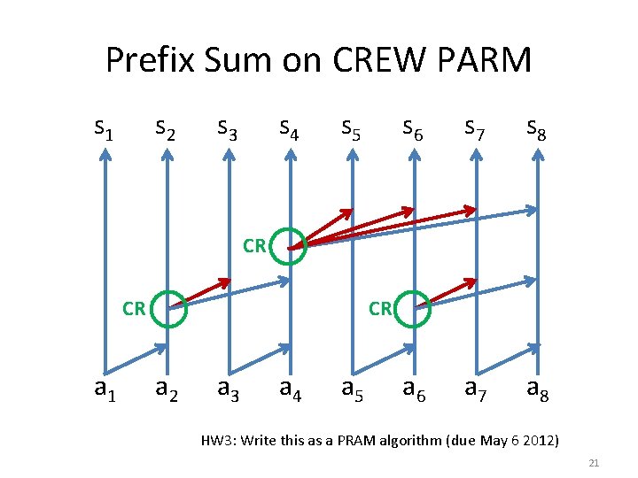
Prefix Sum • 20

Prefix Sum on CREW PARM s 1 s 2 s 3 s 4 s 5 s 6 s 7 s 8 a 6 a 7 a 8 CR CR CR a 1 a 2 a 3 a 4 a 5 HW 3: Write this as a PRAM algorithm (due May 6 2012) 21

Is PRAM implementable? • Can be an ideal model for theoretical algorithms • Algorithms may be converted to real machine models (XMT, Plural, Tilera, …) • Or can be implemented ‘directly’ • Concurrent read by detect-and-multicast • Like the Plural P 2 M net • Like the XMT read-only buffers • Concurrent write how? • • • 22 Fetch & Op: serializing write Prefix-sum (f&a) on XMT: serializing write Common CRCW: detect-and-merge Priority CRCW: detect-and-prioritize Arbitrary CRCW: arbitrarily…

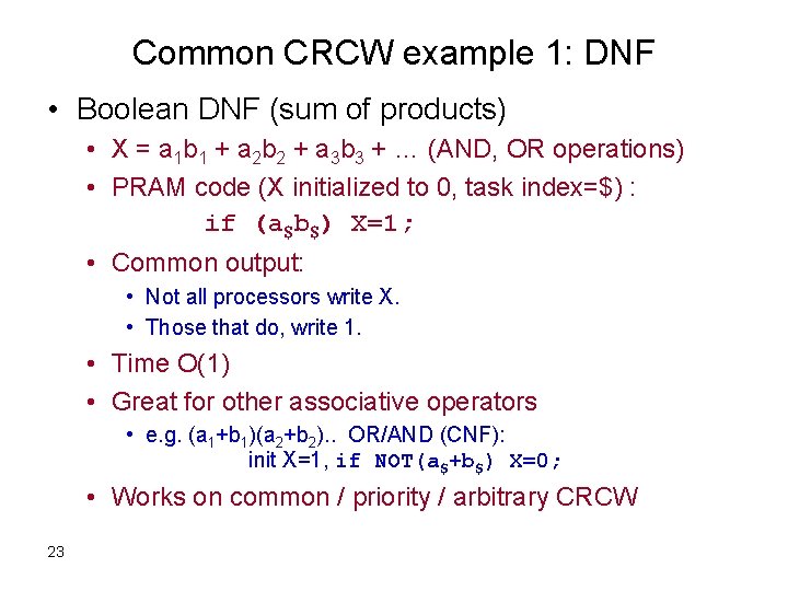
Common CRCW example 1: DNF • Boolean DNF (sum of products) • X = a 1 b 1 + a 2 b 2 + a 3 b 3 + … (AND, OR operations) • PRAM code (X initialized to 0, task index=$) : if (a$b$) X=1; • Common output: • Not all processors write X. • Those that do, write 1. • Time O(1) • Great for other associative operators • e. g. (a 1+b 1)(a 2+b 2). . OR/AND (CNF): init X=1, if NOT(a$+b$) X=0; • Works on common / priority / arbitrary CRCW 23

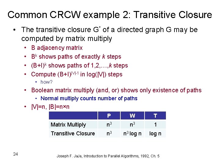
Common CRCW example 2: Transitive Closure • The transitive closure G* of a directed graph G may be computed by matrix multiply • • B adjacency matrix Bk shows paths of exactly k steps (B+I)k shows paths of 1, 2, …, k steps Compute (B+I)|V|-1 in log(|V|) steps • how? • Boolean matrix multiply (and, or) shows only existence of paths • Normal multiply counts number of paths • |V|=n, |B|=n×n 24 P W T Matrix Multiply n 3 1 Transitive Closure n 3 log n Joseph F. Ja, Introduction to Parallel Algorithms, 1992, Ch. 5

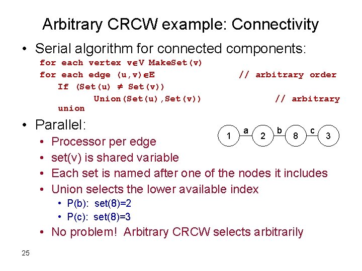
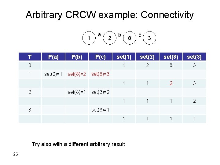
Arbitrary CRCW example: Connectivity • Serial algorithm for connected components: for each vertex v V Make. Set(v) for each edge (u, v) E If (Set(u) Set(v)) Union(Set(u), Set(v)) union • Parallel: • • // arbitrary order // arbitrary 1 a 2 b 8 3 Processor per edge set(v) is shared variable Each set is named after one of the nodes it includes Union selects the lower available index • P(b): set(8)=2 • P(c): set(8)=3 • No problem! Arbitrary CRCW selects arbitrarily 25 c

Arbitrary CRCW example: Connectivity 1 T P(a) P(b) a 2 P(c) 0 1 2 3 set(2)=1 set(8)=2 set(8)=1 b 8 3 set(1) set(2) set(8) set(3) 1 2 8 3 1 1 2 3 1 1 1 2 1 1 set(8)=3 set(3)=2 set(3)=1 Try also with a different arbitrary result 26 c

Why PRAM? • Large body of algorithms • Easy to think about • Sync version of shared memory eliminates sync and comm issues, allows focus on algorithms – But allows adding these issues – Allows conversion to async versions • Exist architectures for both – sync (PRAM) model – async (SM) model • PRAM algorithms can be mapped to other models 27